Fig 2.1 Befunge
(Chris Pressey, 1993)
(Chris Pressey, 1993)
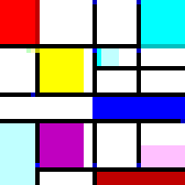
Fig 2.2 Piet
(David Morgan-Mar, 2016)
(David Morgan-Mar, 2016)
Lingdong Huang
Programming languages are systems of notations for writing computer programs, and are important and powerful interfaces for human-computer interaction. The design of a programming language plays a large role in the way the programmer reason about algorithms, and computation in general. Therefore, even though all Turing-complete languages can in theory complete the same set of computational tasks, and that major existing languages are relatively competent and usable for today’s computing purposes, it is far from meaningless to experiment in the design of novel programming languages that facilitates certain types of computation, or to encourage certain modes of thinking, or to appeal to users of certain backgrounds and ways of working, or to bring new aesthetics and ideas of what computation can possibly be about.
In contrast to common (mis)understanding that programming has to be a technical and rigorous endeavor, drawings are often considered intuitive, expressive, and universal. Be it a diagram to explain a certain situation, a mindless doodle while answering a call, or a caricature of your friend — anyone can make a drawing! Meanwhile, drawings can also carry a lot of information and can even illustrate some complex situations and logic with relative ease. Could the design of programming language draw inspirations from drawings? Could it be possible that writing a computer program would be as simple as making a drawing?
We believe that experiments in this direction would be interesting in exploring the unique properties of drawings as an art form, blurring the boundaries between art and code, opening up possibilities and serve as inspirations in future programming language design.
“Computing” and “drawing” are both deeply historical and loaded terms. Although digital media is often positioned in opposition to the “manual” act of drawing, the broader territory of “computing” includes matters of language, rules, procedures, and orders that are very much compatible with the presence of ink on paper. Indeed, the nature of drawing ― a temporal medium governed by marks that can be precisely defined, but not easily edited―provides welcome structure for computational methods.
― Carl Lostritto, Computational Drawing
The idea of two-dimensional programming languages and that of using freehand inputs are by no means new. Notable inspirations for this thesis include:
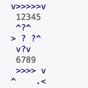
Befunge (Chris Pressey, 1993) is an esoteric programming language that allows arranging a program as ASCII characters in 2D, and the control flow can follow the symbols in four directions.
Piet (David Morgan-Mar, 2016) is a programming language whose programs look like art pieces by the Dutch painter Mondrian. The idea that the representation of a program can “double” as an art piece is inspirational to some of the programming languages presented in this thesis.
|
Fig 2.1 Befunge
(Chris Pressey, 1993) |
Fig 2.2 Piet
(David Morgan-Mar, 2016) |
Dynamicland (Bret Victor, 2018) is an example of “paper computing” where computation is done through manipulation of physical objects and markers, read with cameras and augmented with projectors. The interaction methods in this thesis draws inspiration from this project.
Sonic Wire Sculptor (Amit Pitaru, 2009) is a software that allows making musical compositions interactively by drawing lines in a rotating 3D space. The playfulness and the intuitiveness in the interaction is also a one of the goals for the languages designed in this thesis.
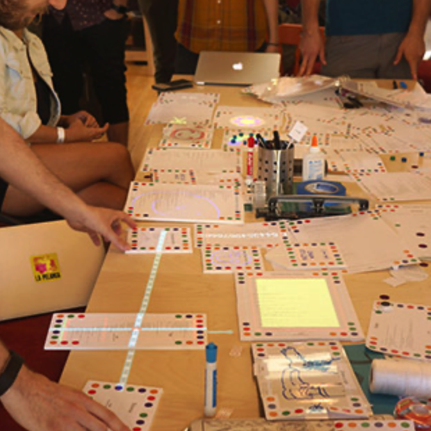
Fig 2.3
Dynamicland (Bret Victor, 2018) |
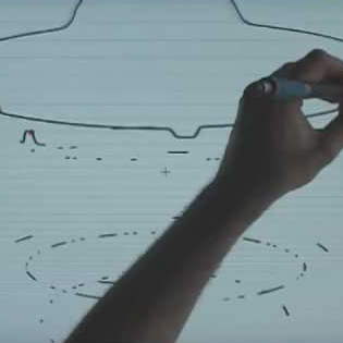
Fig 2.4
Sonic Wire Sculptor (Amit Pitaru, 2009) |
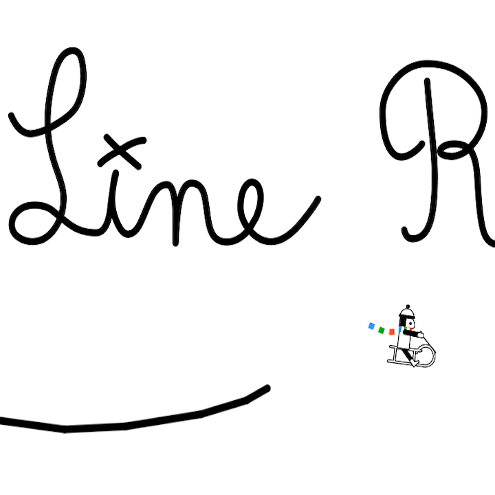
Fig 2.5
Line Rider (Boštjan Čadež, 2006) |
Line Rider (Boštjan Čadež, 2006) is a game in which the player can freely draw “tracks” for the character to slide on. Over the years, many creative (and convoluted) player designs emerged, exhibiting some computation-like properties, which are inspirational to this thesis.
Features of a programming language, whether syntactic or semantic, are all part of the language's user interface. And a user interface can handle only so much complexity or it becomes unusable.
― Guido van Rossum, Language Design Is Not Just Solving Puzzles
The following questions are considered while designing the programming languages described in the thesis. While not all the languages attempt to answer all the questions, they're what the author believed to be important objectives, and are used as metrics for evaluation toward the end of this thesis.
Additionally, the following constraints are used to guide the design process:
While the feasibility of parsing programs from a piece of paper (or a raster image in general) is an important consideration in the design of the languages, the actual development of sophisticated computer vision algorithms is not a major focus for this thesis. Nevertheless, most languages described in the thesis include a section detailing some baseline computer vision techniques to achieve varying level of accuracy, and potential improvements to maximize the accuracy; The practicality of implementing such algorithms is also evaluated.
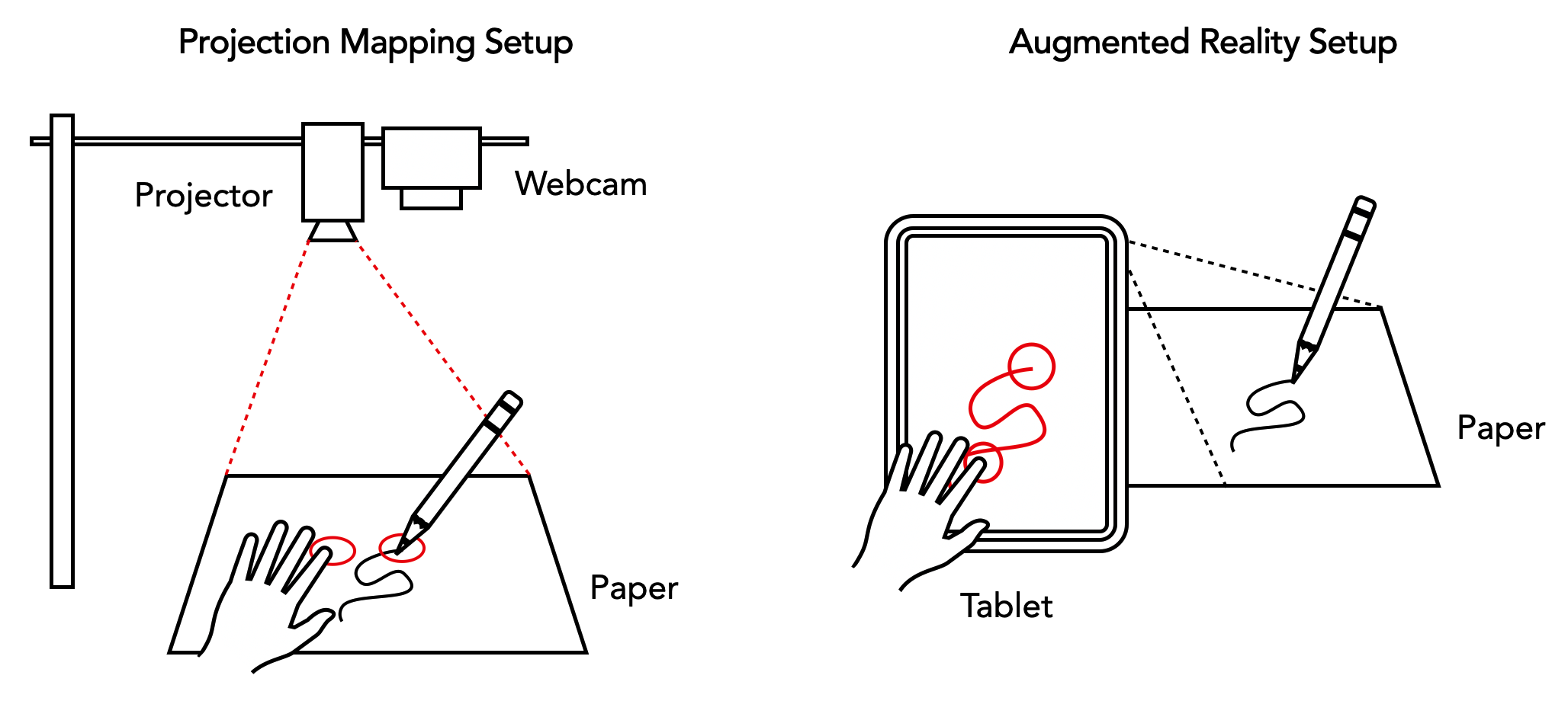
While there is a variety of ways a language implementation can read its input and output, the below illustrated "projection mapping" and "augmented reality" setups are considered optimal ways to experience some of the programming languages described in this thesis:
With these goals and constraints in mind, three main languages (or family of languages) are designed for this thesis, as well as several smaller, "sketches" of languages, experimenting on properties of drawings and their computational aspects.
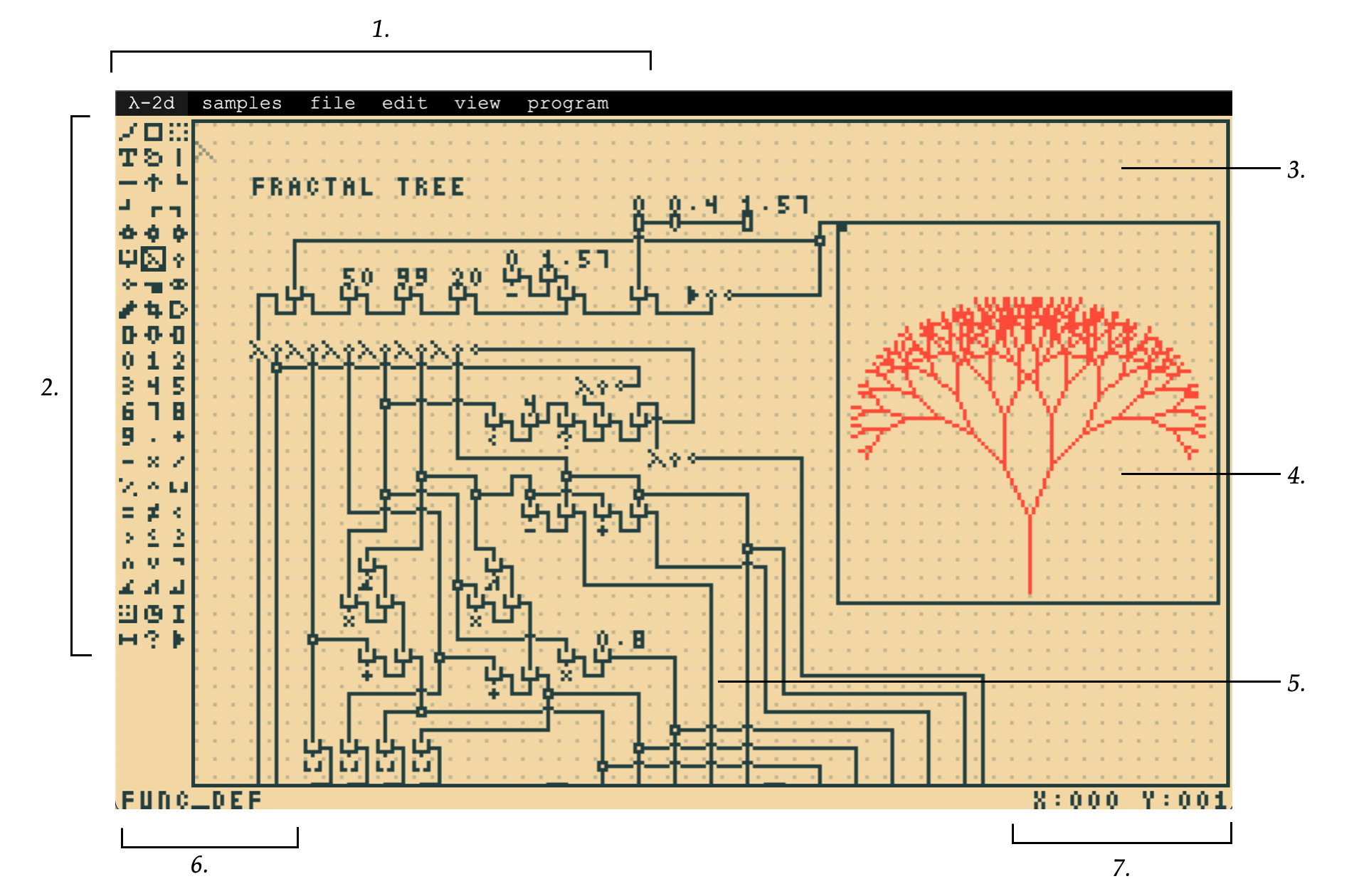
λ-2D is a 2-dimensional, grid-based programming language based on ideas from lambda calculus. The benefit of using a functional paradigm is that functional programs are essentially "expressions" without a pre-determined order of execution, just like how parts of drawings can often be viewed in arbitrary order while in combination construct a certain scene or tell a certain story. By imposing a Cartesian grid, it facilitates parsing of the program (each cell can be recognized as a symbol, and has a fixed neighborhood) as well as clarity and organization, at the price of limiting full freehand expression.
A λ-2D program consists of "symbols", "wires", (and optionally freehand drawings and comments). A symbol is a predefined pattern that denotes an operation, a function, a value, or a variable. The wires connects the symbols to construct meaningful programs, allowing the result of one computation to "flow" into the input of another. Freehand drawings can be used as bitmap inputs for programs to manipulate, leveraging the "drawing-based" nature of the language. Lastly, everything that is not parsed as above are treated as comments, allowing the programmer to draw textual as well as graphical annotations for their code.
Though [lambda calculus] was much less obviously a fully comprehensive mechanical scheme than was Turing's, it had some advantages in the striking economy of its mathematical structure.
― Roger Penrose, The Emperor's New Mind
Like lambda calculus, there are two fundamental "units" in λ-2D: that of function definition and that of function application; everything else derives thusly. While λ-2D has many other constructs to facilitate programming, these fundamental units can be denoted as such:
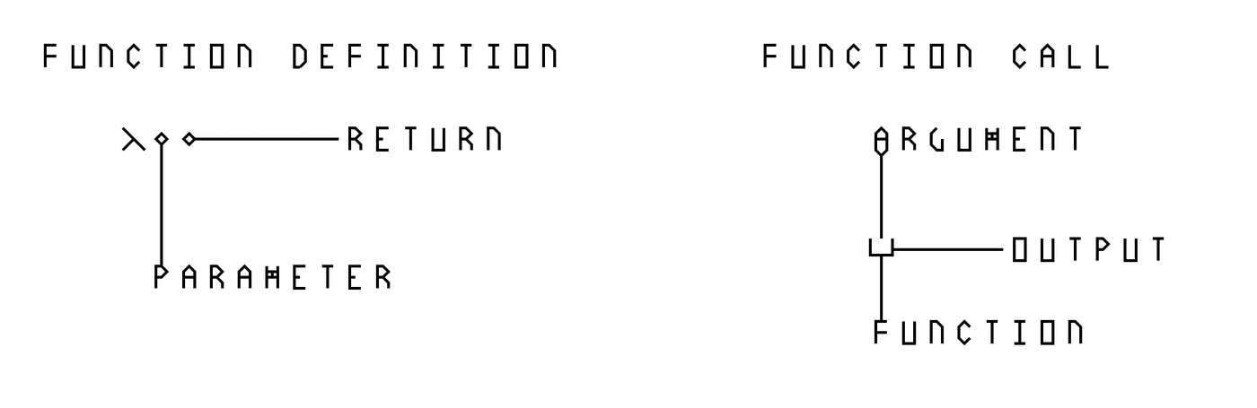
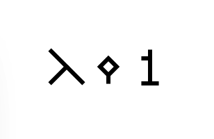
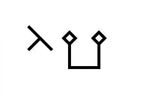
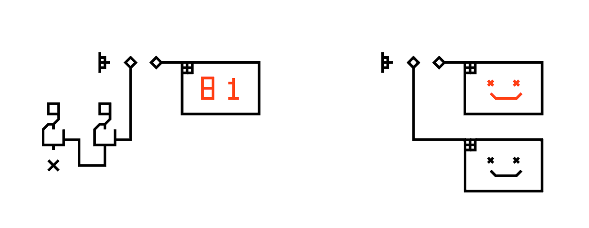
To define a function, the greek letter λ is drawn in the first cell, and in the cell to its right, the single argument (which, by connecting it to other cells via wires, can be referenced by value), and the next cell to the right, the return value. Therefore, the simplest function, which receives a dummy argument and always return 1 (λx.1) can be written as follows:
The symbol of a small circle with a stub of a wire (either on its bottom or to its right) denotes the start or end of the wire. Through a wire connection, a function that always returns its argument (identity function, λx.x) can be written as follows:
The function application syntax uses a "cup" symbol, for the intuition that calling a function is like putting the argument into a box and getting the result spit out. The function reference is connected to the bottom of the symbol, while the argument is drawn on the top (either directly or referenced through wires) and the output can be referenced by connecting a wire to the right of the symbol.
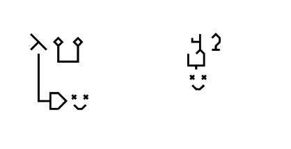
A function always take one argument and return one value. To take more arguments (as is familiar in most programming languages), a technique known as "currying" is used: A function that takes three arguments, is equivalent to a function that takes one argument, and returns another function, which takes another argument, and returns yet another function, which takes the third argument. Currying is expressed in λ-2D as follows:
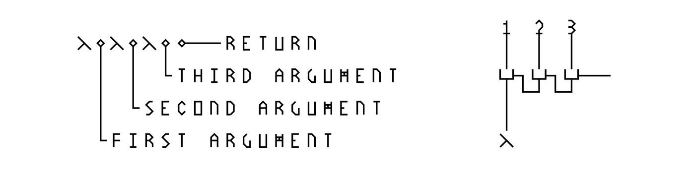
While the logic behind currying is recursive, λ-2D, following the design of many other functional programming languages, allows expressing it in a "flat" manner, so the end-programmer can almost just draw it as a repeating pattern, without thinking each time about "a function that returns another function that returns...". The design also simplifies the syntax of the language, avoiding introduction of additional symbols.
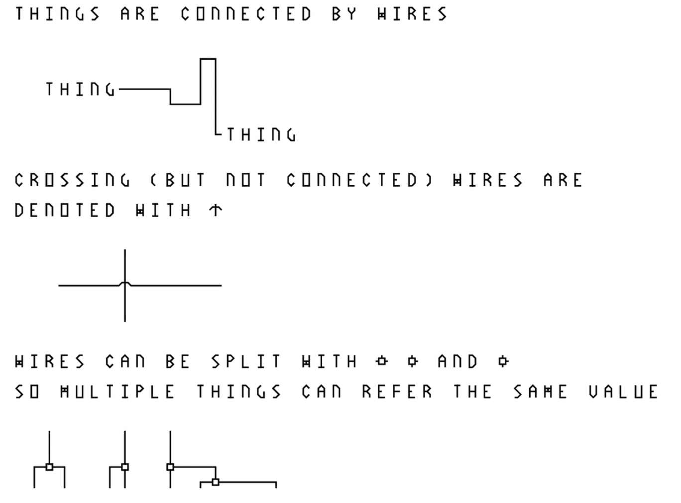
As shown briefly above, wires are used to connect inputs and outputs, to "flow" the data. Wires can cross each other without interfering (jumps) or be split (joints), so that multiple operations can reference the same value. The wires, though unmarked as such, have an implied direction (cells that generates values forward to those that receive them, and never backward). To facilitate parsing as well as for clarity, the joints must be drawn so that the input is on the top, while outputs can either be at the bottom or to the sides. This way, when parsing follows a wire into a three-way intersection, it needs not parse both paths and determine which one provides the value, while the other one is merely another receiver which also reference this value. This would prevent much overhead when a value is frequently referenced multiple times through recursive joints. Other than this, either end of a wire does not have positional requirements (value can flow from right to left, or vice versa) and the wires can be of any length and form any shape.
To reference a function, connect a wire either to the top or bottom of the λ symbol (as its right is already used for argument and output). To reference other values, connect a wire to one of the four von Neumann neighbors of the first (leftmost) symbol of the value (If the value consists of multiple symbols, then the right cell becomes automatically unavailable).
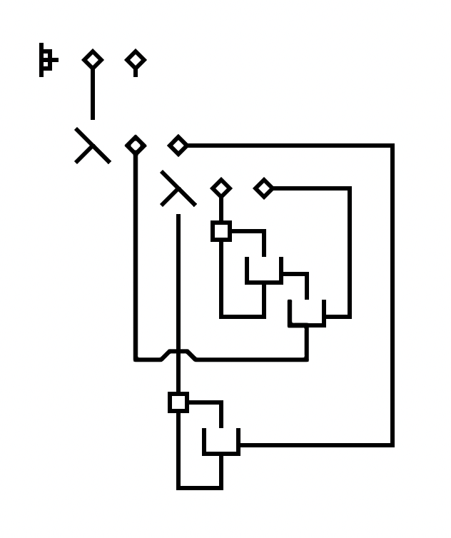
With the constructs introduced thus far, λ-2D is technically Turing-complete, as it is directly translatable from and to lambda calculus. For example, the Y-combinator (λf.(λx.f(x x)) (λx.f(x x))) can be expressed as follows:
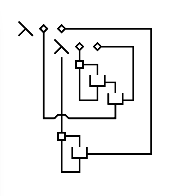
However, to make the language more usable for general purpose, many more constructs are added, such as numbers, arithmetic, math functions and bitmap manipulation. Think of them as the "standard library" of λ-2D.
The built-in numbers does not have a specified encoding (e.g. Church numerals, though users are free to implement their own as such using syntax introduced above), this is so that the underlying language implementation can use whatever that is most efficient or simplest, which in most systems is perhaps the bit-based representation. Real numbers (floating point) are also supported.
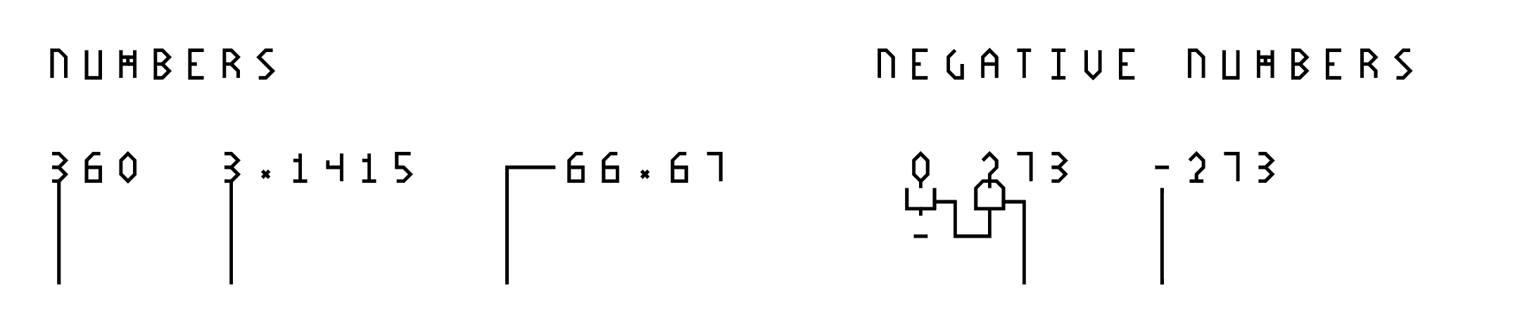
Similarly, a way to write conditional expression is also provided for convenience. The "?" function is defined as follows:
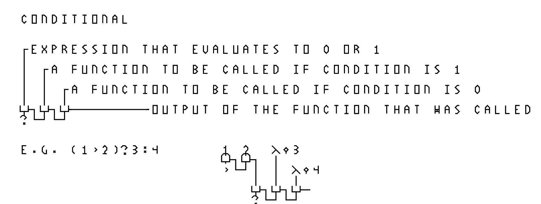
The first argument is the predicate expression, the second is the function to be called when the predicate evaluates to true, and the third is the function to be called when the predicate evaluates to false. The curried function finally returns the result of the function that was called (function IF(p,a,b): if p then return a() else return b()). As the language is purely functional with no side effects, the order of evaluation of these functions (or whether they are evaluated at all when the result is not used) does not matter from the perspective of the implementation.
Frames are special value types that allows definition, manipulation and display of bitmaps (or 2D binary matrices). While "modification" of pixels is inherently violates the functional paradigm, λ-2D circumvents this restriction by defining the "drawing" of a pixel not as:
function PIX(B, x, y):
	turn pixel at B(x,y) on
but instead as:
function PIX(B, x, y):
	return a copy of B, with pixel at (x,y) turned on
Similarly, "printing" the execution result of a program can be thought of as returning a bitmap with certain pixels turned on, such that the bitmap has certain patterns that resembles "text" to the speakers of a certain language. In fact, this is the standard method of output of λ-2D. As a purely functional language, no assumption can be made about "execution order", so a series of conventional "print statements" would only yield garbled output; Moreover, each print statement would always print the same result, as there are no state changes that could affect the value of an entity over time. Details on program entry point and displaying outputs will be discussed later.
To define a frame, a special symbols is used for the upper left corner, while the remainder of the frame are drawn as a rectangular enclosure made of regular wires.
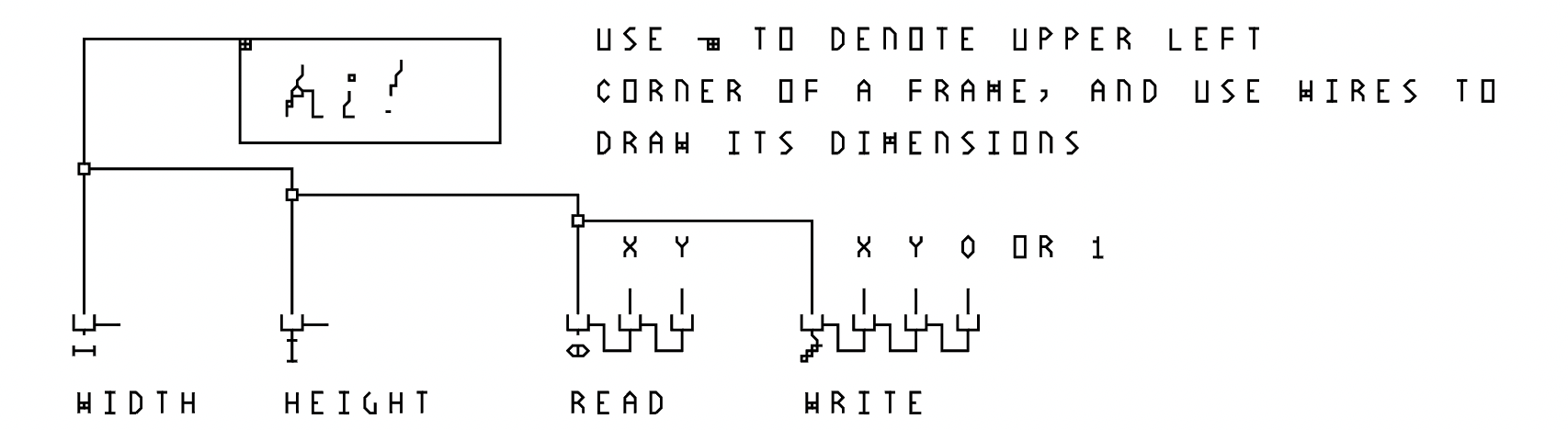
User can define frames of arbitrary dimensions, as long as the width and height are multiples of the grid size. For example, in the reference implementation of λ-2D, each grid has a resolution of 5x5 pixels, so frame dimensions can be 5x5, 10x15, 640x480, etc.
Inside the frame, the user can make freehand drawings, which can be used as inputs to the program. Or, they could use it as a matrix (or array) of bits to store data. The "pixel read" and "pixel write" function shown above are used to detect and update the pixels.
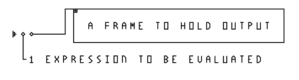
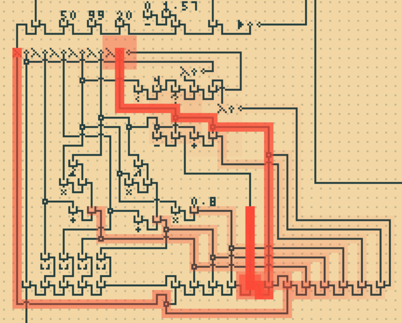
Program entry point is defined using a rightward-pointing triangle, reminiscent of the "play" button on common interfaces. In the neighboring cell to the right of the entry point is an expression to be evaluated upon program start, and the next cell to its right leads to a frame which should be used to hold the output of the program after it is run. A λ-2D implementation should attempt to display the output directly in that frame, if on a digital/screen-based interface, or through projection or other means when on a physical interface. Only at this final moment, the functional idealism clashes with the imperative nature of reality, and the inevitable state change is manifested (as the pixels on the user's screen change color). The user can assign an area of arbitrary position and size within the representation of their program for storing output.
To avoid a program from becoming a great tangle of wires, "labels" can be used to name entities. Think of them as variable names; but instead of using a string of ASCII characters, the user can design custom symbols. To define a label, connect an entity to the "⌂" symbol, and draw the custom shape to its left. This custom shape can now be used in place of the original entity.
In addition to constant values, the user can also use dynamic "sliders" as input. The slider body consists of an arrangement of 4 symbols. To the left, it must start with the track-begin symbol, followed by a number of horizontal wires, followed by the slider-thumb, and again a series of horizontal wires, and ended on the right by the track-end symbol. Above the slider, the min/max/current values are labeled with numbers. To use the slider, one must connect a wire from the referencer to the track-begin symbol.
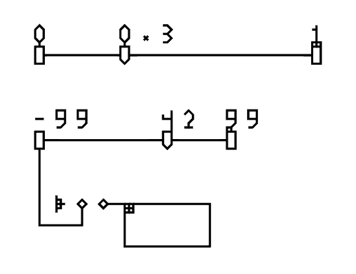
The numerical label on the slider thumb serves as the default value. The position of the thumb does not need to be accurate (and in most cases, cannot be), and the number above it solely determines the value. However, a decent programmer should draw it roughly at a sensible position.
In an interactive λ-2D implementation, the user would be able to drag the slider along the track to modify its value. This can be either realized a direct modification of the input program, or as an overlay for visual clarity as well as for avoiding destructive editing.
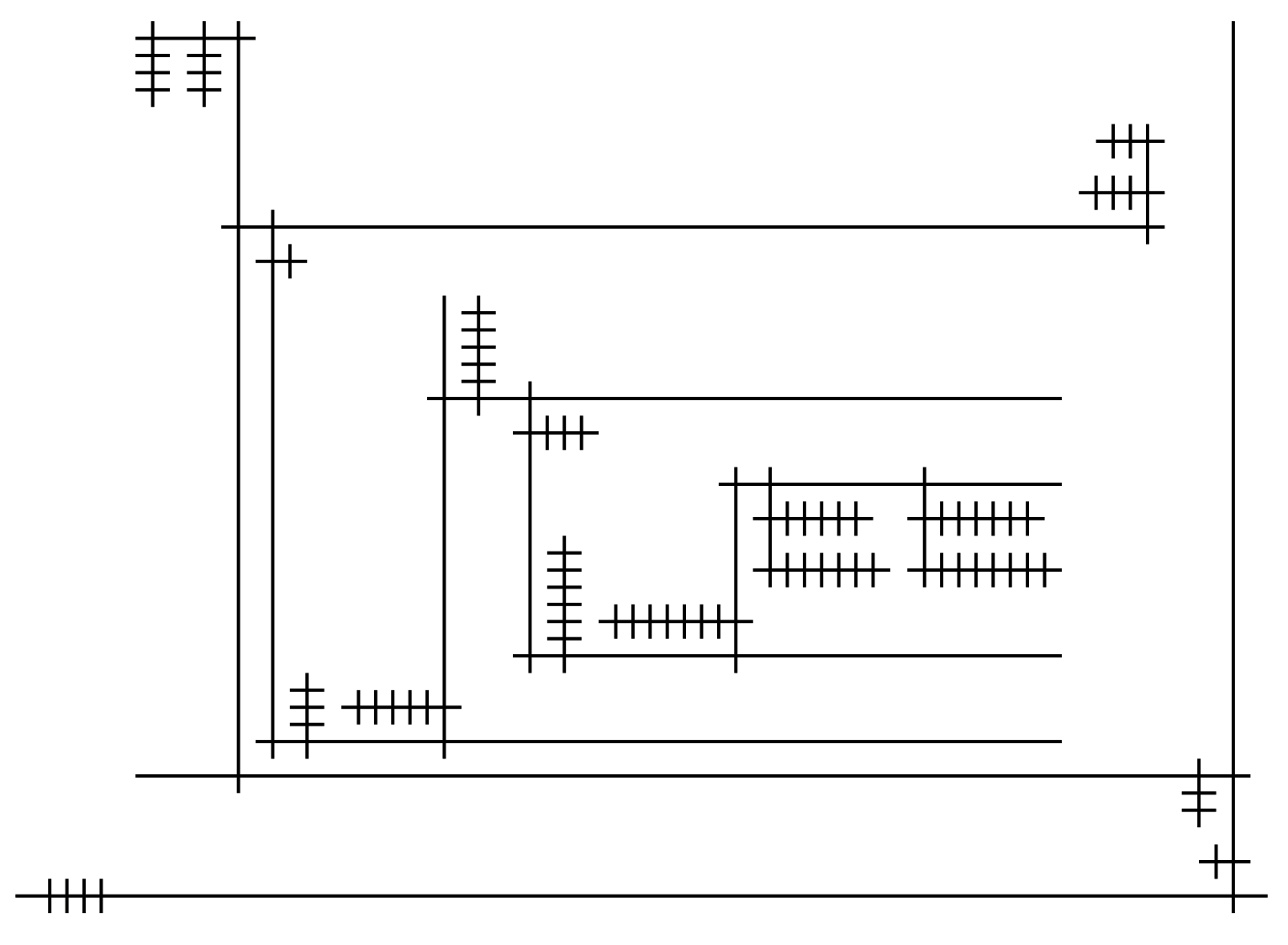
No programming language demonstration can be truly complete without a few code examples. Let's look at a simple recursive factorial program:
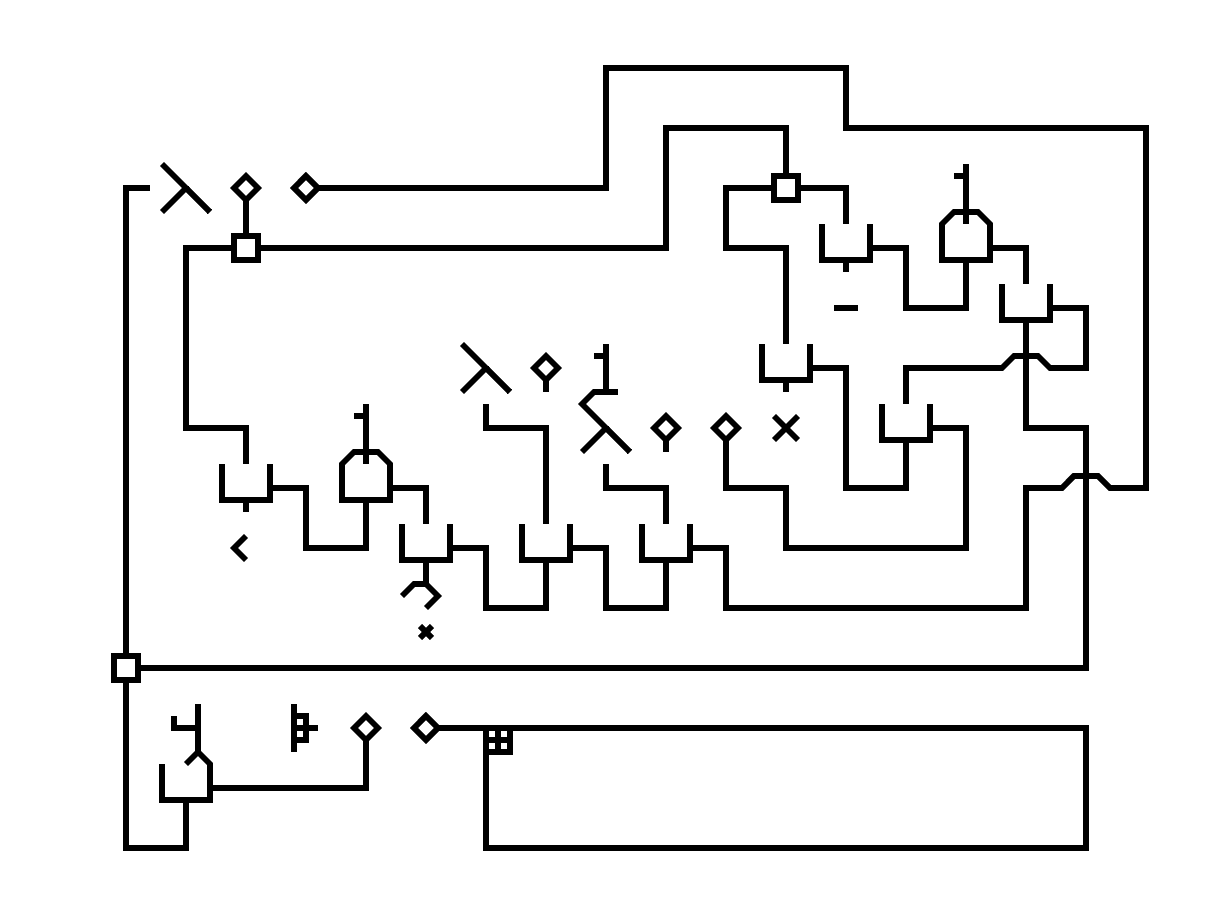
Which translates to the following pseudo-code:
function FACT(x):
	if x < 1 then
		return 1
	else
		return x * FACT(x-1)
print FACT(4)
Each part of the program is dissected and explained below:
|
|
1. The entry point informs us this program involves applying a certain function to the number 4, and printing the result. What function is it? We shall follow the upward-pointing wire... |
|
|
2. We can now see that this is a function that takes one argument. Let's, for the sake of explanation, call the function f, and the argument x. It first checks whether x is smaller than 1, and then do a conditional expression based on the test... |
|
|
3. If the predicate evaluates to true, then the conditional expression would evaluate a function that constantly returns 1 (hence also return 1 itself). Otherwise, it would evaluate another function, which involves multiplying together two "somethings"... |
|
|
4. Following the wire, we see that the first of the two "somethings" turns out to be the argument x we saw earlier. The second "something" is the result of some subtraction. The minuend is also x (notice the joint that allows feeding the same value to two destinations). The subtrahend is the constant value 1. |
|
|
5. The result of the conditional expression is fed to the return cell of the function f. Therefore, the return value of this expression is the final output of the function. Finally, now that we know how f is defined, we can apply it to the number 4 (an incidental choice), as specified by the entry point. |
As you might have noticed, a λ-2D program can look a bit complex at first, but once we're familiar with the way they're drawn, they can be rather fun to work with.
A listing of common symbols (excluding wires, numbers and function definition) can be found below:
 |
Read Pixel (B,x,y) Write Pixel (B,x,y) Crop Bitmap (B,x,y,w,h) Label Slider track left Slider "thumb" Slider track right Add (x,y) Subtract (x,y) Multiply (x,y) Divide (x,y) Modulo (x,y) Power (x,y) Floor (x) Equality test (x,y) Not equal (x,y) |
 |
Lesser than (x,y) Greater than (x,y) Lesser than or equals to (x,y) Greater than or equals to (x,y) Logical AND (x,y) Logical OR (x,y) Logical NOT (x) Cosine (x) Sin (x) Arctan2 (x,y) Random (x) Time: seconds since (x) Bitmap height (B) Bitmap width (B) Conditional (p,a,b) Entry point |
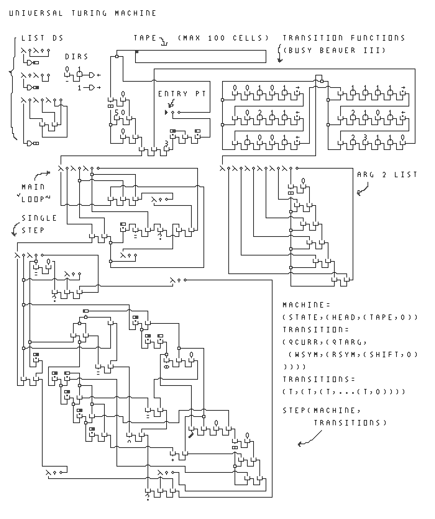
As shown previously, there exists a one-to-one mapping from a subset of λ-2D to lambda calculus, the latter of which is Turing complete. Nevertheless, a universal Turing machine simulator in λ-2D is provided below:
A reference implementation and an integrated development environment (IDE) has been developed for λ-2D. The implementation is a transpiler (translator-compiler) from λ-2D to JavaScript, written in JavaScript, with a web based editor. The editor provides basic functionalities such as creating and running programs, import and export, as well as some strange features such as visualizing and sonifying the execution of a program, or rendering and obfuscating the program in different styles.
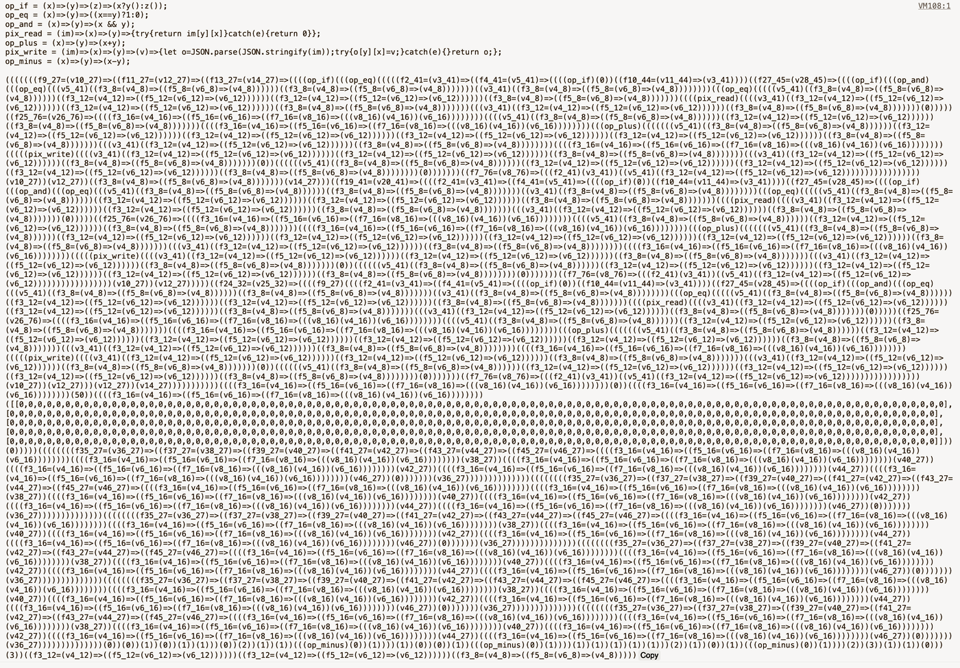
The transpiler was so lazily implemented that one might describe it as a "hack". By leveraging the loose syntax of JavaScript, every λ-2D program can be compiled into a single JavaScript expression ("one-liner"), after which the generated JavaScript output is simply evaluated with the browser built-in eval() function.
The parser starts by looking for the entry point of the program, and then follows the wires, pulling together various symbols as required, which in turn lead to more wires and symbols, and with them reconstruct the program (A "top-down" approach). Functions and their arguments are given temporary names based on their coordinates in the drawing (which we know for sure are unique, and it facilitates debugging as well). It keeps a dictionary of functions that it has already seen by the current branch, to avoid redefining recursive functions endlessly. Since in JavaScript, assignment expressions returns the value assigned (e.g. the value of (x=3) is 3), and assigning to variables without prior declaration is allowed (but makes them globals), the parser is able to define and name functions at the same time, in-line, without declaration.
Below is the pseudo-code for a simplified version of such implementation.
function PARSE_AT(
	P     : map<coordinate,symbol>,
	(x,y) : coordinate
	S     : list<function>
){
	if P[x,y] is a wire endpoint then
		if P[x-1,y] is a λ symbol then
			return "v_{x}_{y}"
		else
			return PARSE_AT(P,FOLLOW_WIRE(P,(x,y)),S)
		end
	else if P[x,y] is a function call then
		a := PARSE_AT(P,(x,y-1),S)
		f := PARSE_AT(P,(x,y+1),S)
		return "({f})({a})"
	else if P[x,y] is a function definition then
		f := "f_{x}_{y}"
		if f is in S then
			return f
		else
			record f in S
			return "({f}=(v_{x+1}_{y}))=>({PARSE_AT(P,(x+2,y),S)})"
		end
	else if ...
		...
	else
		error "Unrecognized Symbol"
	end
}
Where "...{x}..." denotes string interpolation. For the sake of space, the trivial cases of parsing numbers, frames, built-in functions etc. are not included. Upon the calling parser, on, for example the Y-combinator function shown before, the following string will be returned:
(f3_3=(v4_3)=>(((f5_4=(v6_4)=>((v4_3)((v6_4)(v6_4)))))((f5_4=(v6_4)=>((v4_3)((v6_4)(v6_4)))))))
If we clean up the names and parenthesis a bit, the true identity of this function is revealed:
Y=(f)=>((x)=>f(x(x)))((x)=>f(x(x)))
The λ-2D implementation features an interactive WYSIWYG web GUI. Each symbol is implemented as a 5x5 bitmap, which the user can "stamp" onto a "canvas". This strategy simplifies asset creation, and allows the program to be saved as a bitmap image (e.g. in the PNG format), and be loaded from one as well.
A dissection of the editor components is shown below:
The IDE is capable of visualizing the execution of a λ-2D program through animating a "signal" that travels along the wires. In fact it is perhaps more accurate to say it's a visualization of the parsing of the program, as the actual execution is handled by the generated JavaScript, which happens atomically (to the programmer, at least); However, if the implementation were a (tree-walk) interpreter, the visualization of execution would be identical to the current visualization of parsing, so it isn't entirely false advertising.
The animation does not happen synchronously with the parsing; Instead, as the program is parsed, the order of cells that were visited is recorded, and the sequence is used to drive the playback after the parsing is finished. This minimizes the overhead in both passes, and allows them to run independently of one another.
In addition to leaving a trace, the animated signal also makes a noise as it passes through each symbol, the pitch of which is determined by what the symbol is. The resultant "score" somewhat resembles game music from the 8-bit era (as the sounds are generated with a simple oscillator). Since each symbol makes a distinct sound, it is theoretically possible for a person with acute hearing (as well as fast brain processing speed) to "read" a program by listening to the score. It is also theoretically possible for the musically talented to compose a program that both sounds nice, and do something interesting.
While this implementation is bitmap-based (symbols are made of tiny pixel art), it is possible to trace the bitmap automatically to produce a vectorized, line-based representation. This allows reproducing the program at arbitrary scale without the pixelated look, as well as CNC-plotting the program on paper. In fact, the figures shown in previous sections are produced using this tracing algorithm. The algorithm can be summarized as follows:
function TRACE(B):
	for each (x,y) in B do
		b := {0,0,0,0}
		if B(x,y-1) then
			flip b[0], b[1]
			ADD_LINE((x,y), (x,y-1))
		end
		if B(x,y+1) then
			flip b[2], b[3]
			ADD_LINE((x,y), (x,y+1))
		end
		if B(x-1,y) then
			flip b[0], b[2]
			ADD_LINE((x,y), (x-1,y))
		end
		if B(x+1,y) then
			flip b[1], b[3]
			ADD_LINE((x,y), (x+1,y))
		end

		if (not b[0]) and B(x-1,y-1): ADD_LINE((x,y),(x-1,y-1))
		if (not b[1]) and B(x+1,y-1): ADD_LINE((x,y),(x+1,y-1))
		if (not b[2]) and B(x-1,y+1): ADD_LINE((x,y),(x-1,y+1))
		if (not b[3]) and B(x+1,y+1): ADD_LINE((x,y),(x+1,y+1))

		if no line has been added for current pixel:
			ADD_LINE((x-1,y-1), (x+1,y+1))
			ADD_LINE((x-1,y+1), (x+1,y-1))
		end
	end
end
The key of the algorithm is to solve the following exemplary issue: given a 3x3 "+" shape shown below, if we consider the Moore (8-) neighborhood, then the traced lines would contain a diamond shape (in addition to the desired cross shape). This arguably would contrast with our expectation. However, it is equally problematic to only consider the von Neumann (4-) neighborhood, since this time the slash "/" shape wouldn't be connected properly.
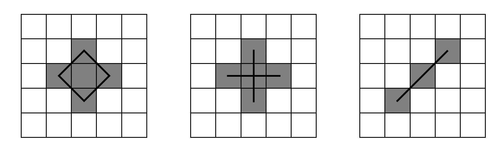
Therefore, the heuristic is simply to consider the von Neumann neighborhood first, and for each von Neumann neighbor found, "block" or "disable" the consideration of Moore neighborhood in its ±45° directions. Only secondly do we consider the Moore neighborhood for those positions that have not been blocked. Thirdly, if neither neighborhood exist, draw a tiny cross to represent a "dot".
After finding all segments, connect all that have ends that meets.
This heuristic seems to work well enough on λ-2D programs, though there are still a few imperfections, as are evident in figures shown in the previous section. However, since the interpretation of pixel art very much depends on the imagination of the artist and the viewer, there's only so much a simple and deterministic algorithm can do.
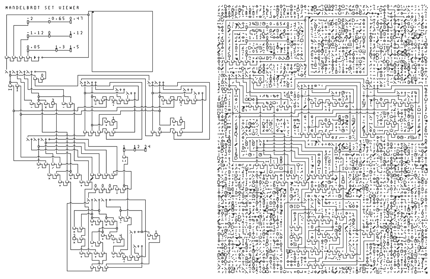
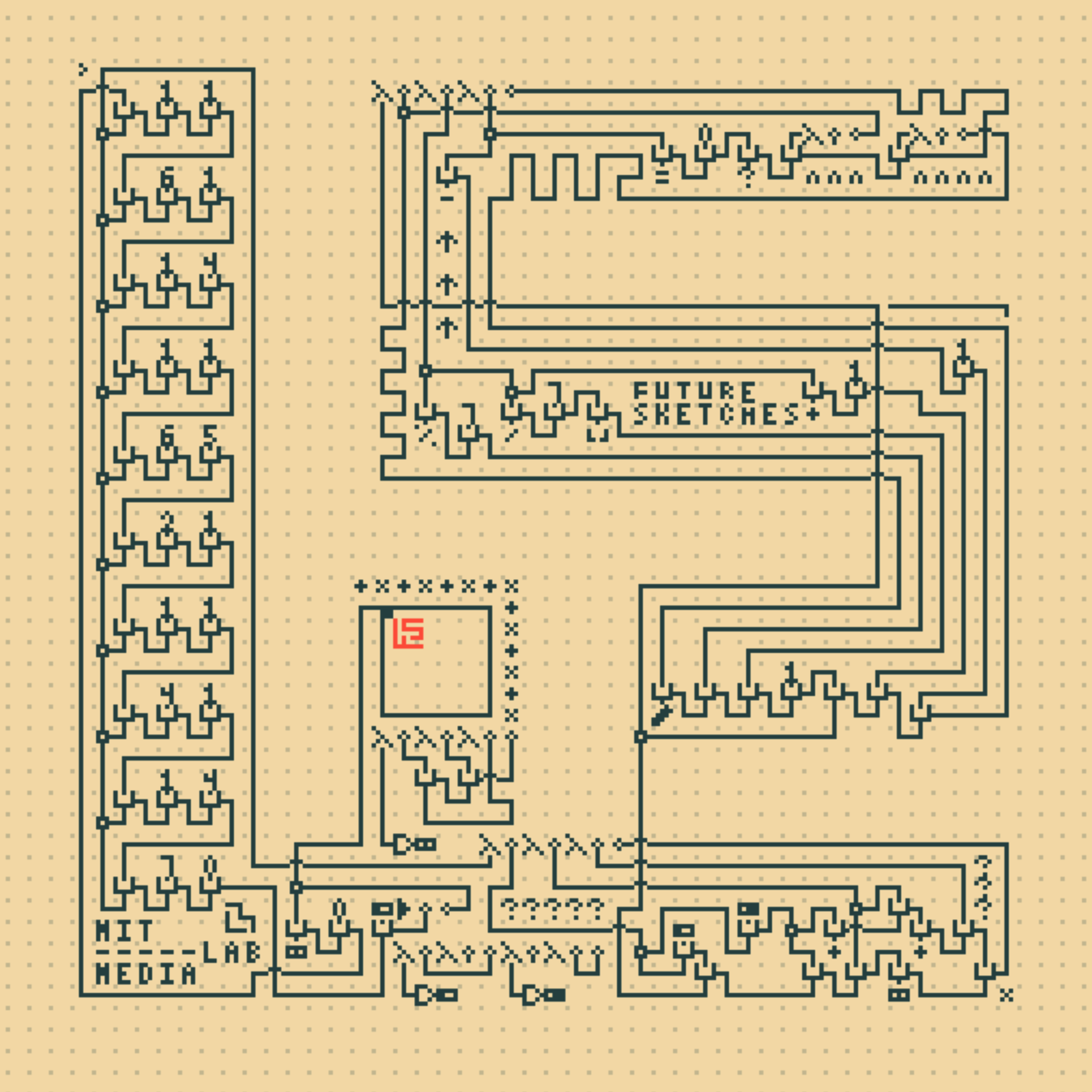
This implementation is also capable of automatically decorating (obfuscating) a program. Since anything that is not reachable by the entry point via wires is ignored, anything can be drawn on the "negative space" surrounding a program (including confusing symbols). Two obfuscation schemes are offered by default: Hieroglyphic and Labyrinthian.
A scheme for extracting a λ-2D programs from a piece of paper using simple computer vision techniques is given below:
Programs must be drawn or printed on a piece of paper with arUco markers on four corners. The dimensions of the paper must be a multiple of the grid size, and be known beforehand.
After the arUco markers are detected, compute the homography matrix and use perspective transformation to straighten the image. Optionally apply preprocessing such as adaptive thresholding or contrast adjustments. Finally, divide the image by the known grid size, and for each grid, find the closest matching symbol in library.
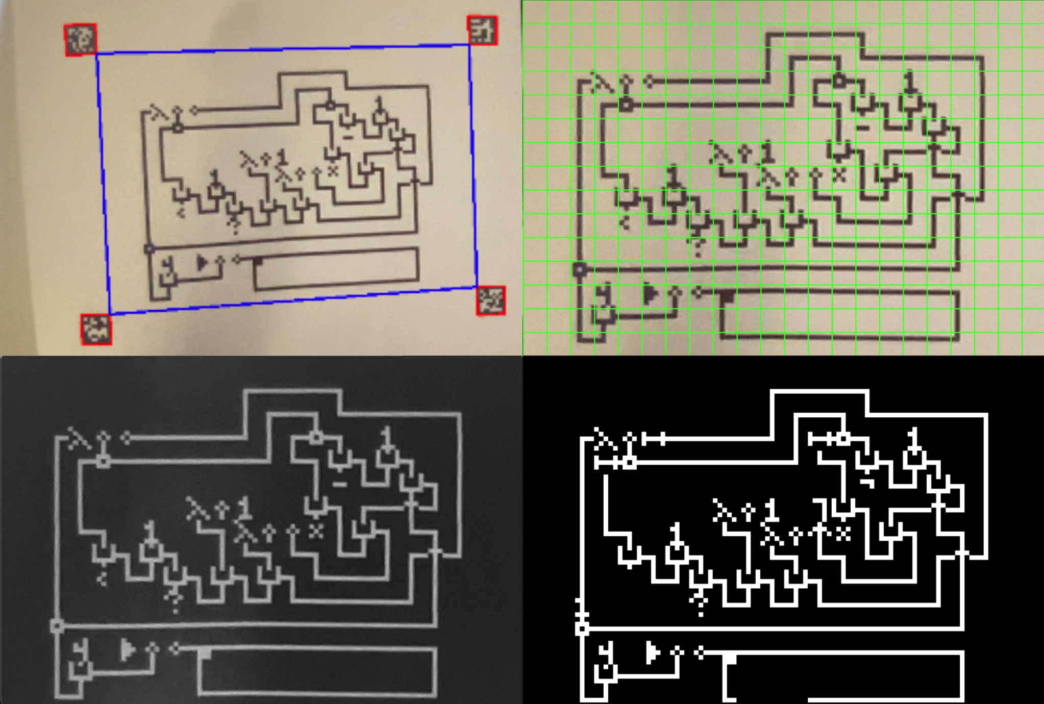
This scheme can parse printed λ-2D programs somewhat accurately. However, even one or two incorrect symbols would be produce an erroneous program. The accuracy would further decrease if the program is hand-drawn.
To achieve more accurate parsing, one could introduce some sort of redundancy or error checking/correction code. However, this would incur an inconvenience on the user. Alternatively, one might train a deep neural network to detect the program automatically. If an algorithm detects each symbol individually, one could further improve the accuracy by filtering out candidates that would've resulted in a syntax error (assuming the input program is correct).
As λ-2D programs have much structure and a limited set of symbols, it is perhaps safe to say that given today's technologies, a satisfactory computer vision algorithm could exist; However, it is not the focus of this thesis to develop such algorithms, though the feasibility of which is considered as part of the designs.
λ-2D makes extensive use of symbols ― and it can perhaps be said, that symbols are only one step away from characters and words. In this sense, λ-2D stands on the bridge between the land of text-based programming language and that of drawings: is it possible to design languages that make use of inherent properties of drawings, such as transformations and topologies of lines and shapes, instead of relying on symbols as an agent?
Nor-Wires, and several other languages were conceived in the quest of answering this question.
Bits also play a part in logic, that strange blend of philosophy and mathematics for which a primary goal is to determine whether certain statements are true or false. [...] Programming in machine code is like eating with a toothpick. The bites are so small and the process so laborious that dinner takes forever.
― Charles Petzold, Code
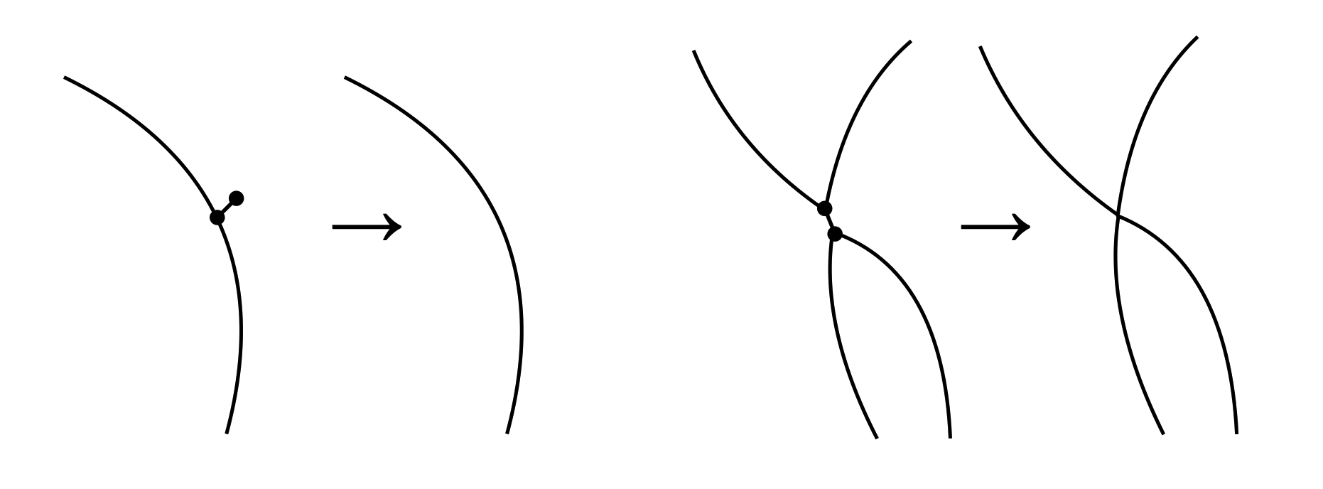
A Nor-Wires program consists of a tangle of interweaving "wires" that carry boolean "signals". The wires intersect one another and join at end points. Call such joining of end points "nodes". Each node must have exactly three incident wires. If the incident wires of a node forms shape of the letter "Y" (two wires from above, one wire from below), it denotes a NOR gate. If the node instead resembles the shape of the letter "λ" (one wire from above, two wires from below), it denotes a "fork". The wires may intersect with each other; These intersections are easily distinguished from nodes, as they cannot have three incident wires (by endpoint-exclusive definition of "intersecting"). The nodes and intersections do not need to be marked by, for example, enlarged "dots", though they could be, if so eases visual clarity. Therefore neither would points with two incident wires have significance, as they would be treated as a part of a continuous wire.
A "NOR" node take the signal from the two wires coming from above, computes the NOR of these two boolean signals, and output the resultant signal to the wire below.
A "fork" node takes the singular signal coming from above, duplicates it, and outputs to both of the wires below.
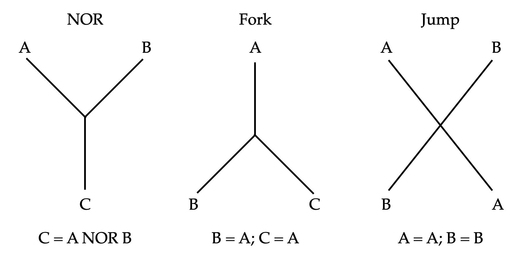
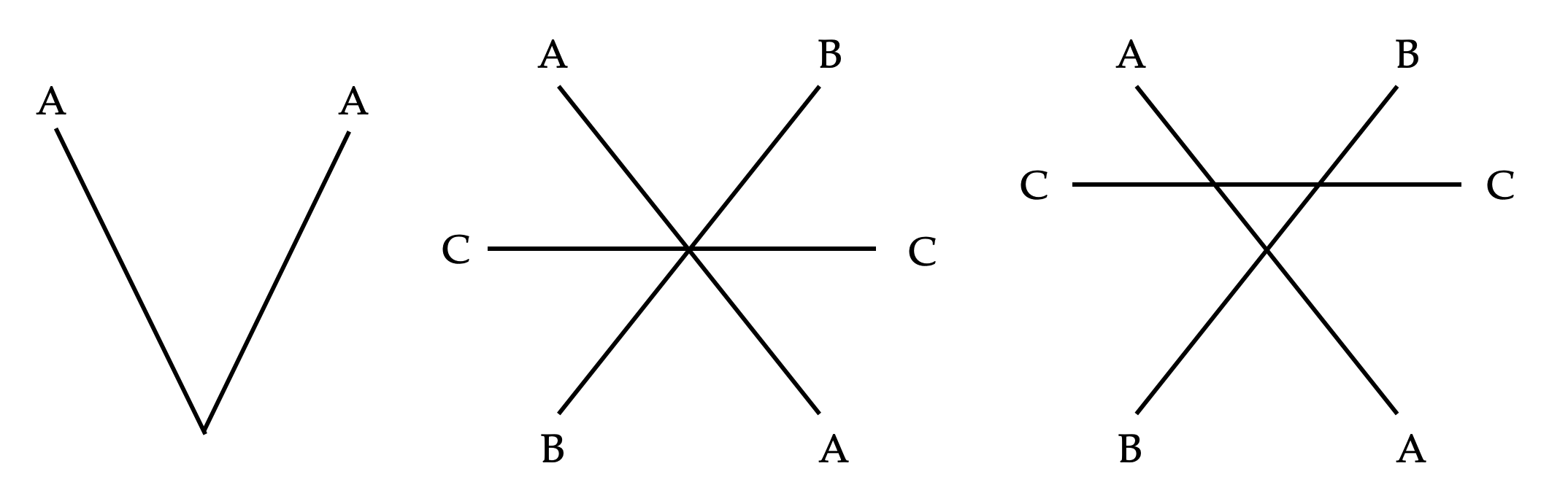
As opposed to the nodes, intersecting wires' signals do not interfere with each other: think of them as "jumps". For visual clarity and to ease parsing, it is advisable to "space out" the intersections, such that each intersection is the result of only two crossing wires (though it is possible to parse intersections of higher degree using a heuristic, such as every wire should be matched with one that introduces the least angle change).
A Nor-wire program typically receive input signals from "top" endpoints (whose wires go downward), and returns its output(s) at "bottom" endpoints (whose wires come from above).
The syntax of Nor-wire is neat in two respects. First, by using one universal gate, there is no need to use any symbols to denote any operation: It can be simply inferred from the shape formed by the incident wires. Even so, there still needs to be a way to feed multiples of the same signal to multiple NOR gates; and the fork node, which coincidentally require one input and two outputs, becomes a perfect symmetry of the NOR node. Second, the non-planar graph parsing/visualization problem (is it a jump, or is it a node?) is solved automatically without need for special marking (such as a tiny "dot" or "bridge"), since all node must be of degree three, and everything else are not connected. These attributes allow Nor-wire to be minimalistic in design, and simple for computer algorithms to parse robustly.
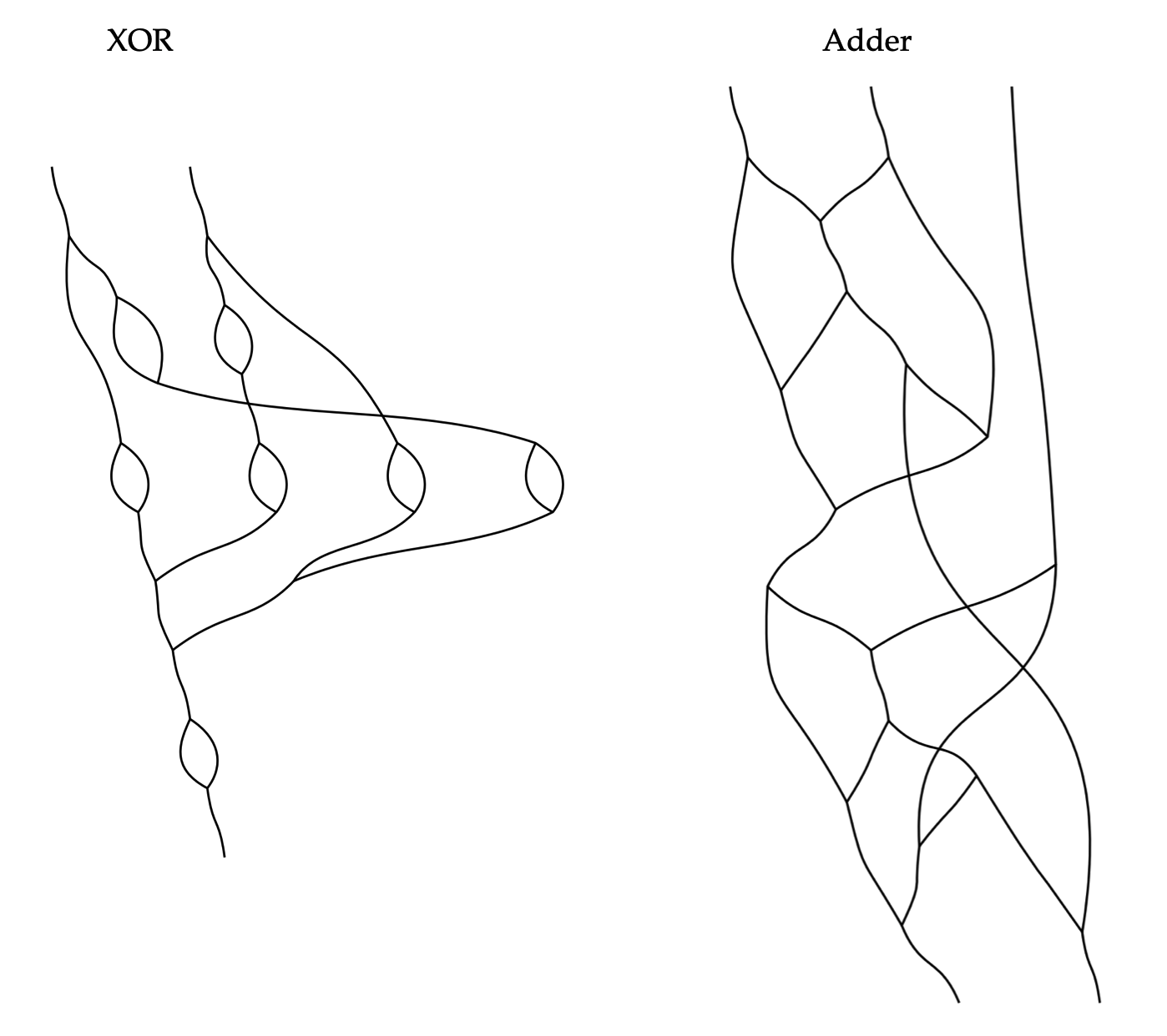
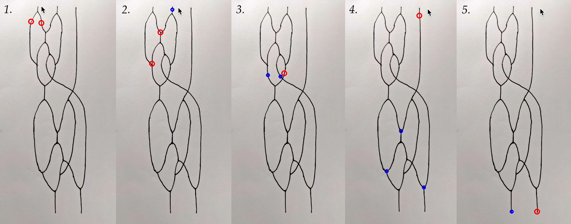
As the AND, OR, NOT gates can be constructed from NOR gates, so can they be from Nor-Wires. Below are example constructions:
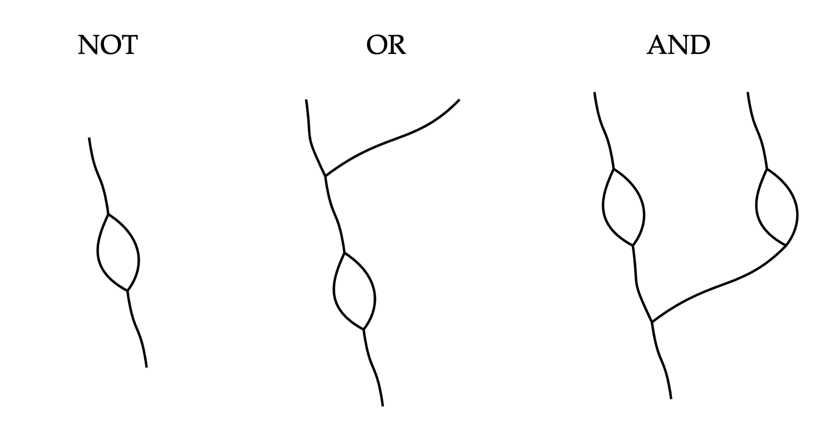
Slightly more complex examples, such as XOR and the full adder, are given below:
A baseline implementation for Nor-Wires is described below, which includes features such as click-and-drag editing, generating a Nor-Wires program from a text-based notation, parsing hand-drawn programs via webcam, animated execution of programs, and several rendering options.
To facilitate development and understanding of Nor-wire programs a simple "assembler" is made to compile a text-based notation into graphical nor-wire programs. The syntax of the notation consists of three basic "instructions", as detailed in the Backus-Naur form (BNF) below:
<program>    ::= (<instr> "\n")*
<instr>      ::= <inp-instr> | <out-instr> | <nor-instr>
<wsp>        ::= (" " | "\t")+
<var>        ::= [A-z]+
<inp-instr>  ::= "inp" <wsp> (<var> <wsp>)* <var>
<out-instr>  ::= "out" <wsp> (<var> <wsp>)* <var>
<nor-instr>  ::= "nor" <wsp> <var> <wsp> <var> <wsp> <var>
The "inp" instruction denotes the input of the program, which starts with the word "inp" followed by an arbitrary number of variable names, delimited by space. The "out" instruction denotes the output, and similarly, starts with the word "out" followed by a list of variable names. The "nor" instruction takes exactly three positional arguments: the output variable name, the first input variable name, the second variable name, in that order. Here is an example:
inp a b c
nor d a b
nor e a d
nor f b d
nor g e f
nor h g c
nor i g h
nor j h c
nor k i j
nor l h d
out k l
For convenience, the macros "and", "or" and "not" are introduced. The syntax is similar to "nor", and the assembler would automatically expand them to a construction made of "nor". For example:
inp a b
or  c a b
out c
expands to:
inp a b
nor tmp a b
nor c tmp tmp
out c
The first argument of "nor", "not", "and" "or" is always the output, followed by input(s). The actual name of the "tmp" variable would've been generated at compile-time.
Notice that the "fork" node in Nor-Wires is implicit in the text notation. By using a variable of a certain name multiple times across different parts of a program, forks are automatically generated, recursively if need be, by the assembler.
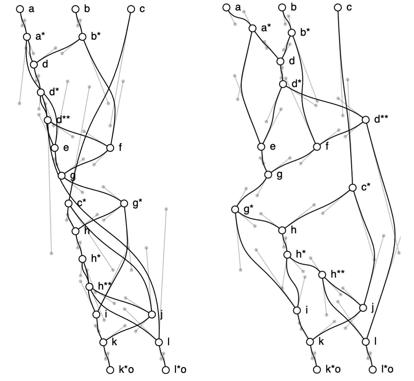
To automatically layout a graphical program based on the text notation, the assembler makes the following observation: If variable c = a NOR b, then c would be most naturally placed at a height below both that of a and that of b. Therefore, as long as the program is not cyclic, every variable (node) can be assigned a "level", or Y-coordinate, based on its dependencies.
function CALC_LVL(k:node, H:list<node>)
	if k in H then return 0
	if k.lvl is defined then return k.lvl
	k.lvl := MIN(1, k.children.map(c=>CALC_LVL(c,H+k)))-1
	return k.lvl
end
n := 0
for each k in nodes do
	n := MIN(n, CALC_LVL(k, []))
end
for each k in nodes do
	k.lvl := k.lvl - n
	if k.type is "inp" then k.lvl := 0
end
The X-coordinate however, is more tricky. Though for a nor-wire program to be valid, nodes of each level could be placed anywhere along the axis; However, ideally, they would be so placed that, there is the least number of intersections. Unfortunately, a naïve algorithm would take factorial time to find an optimal solution; In fact, it has been proved that crossing number is a NP-complete problem, through a reduction to the optimal linear arrangement problem . An approximation is likely to be necessary. One possible approximation is to use randomization; One could perhaps also add local optimizations, swapping the position of two nodes, if so reduces the number of intersections. Force-directed graphs could also be an interesting approach, though the typical goal, which is to space out the nodes, might need to be tweaked.
This baseline implementation does not attempt at such optimizations, however. It would simply space out nodes along the X-axis in the order they are seen, and add a half-phase offset/staggering to each level. The user can then click and drag the nodes freely, until a configuration pleases their eye. They can also manipulate the curvature of the connecting wires using Bézier curve handles.
As stated previously, the minimalism in Nor-Wires' design made it relatively easy for computer vision algorithms to parse robustly from camera image. Since the meaning of a program is derived solely from the topology of the lines, and is invariant to most distortions and warping (excepting a rotation of over 90°), an algorithm wouldn't have to rely on perspective correction and alignments. A scheme for extracting Nor-Wires programs from RGB webcam feed is presented below.
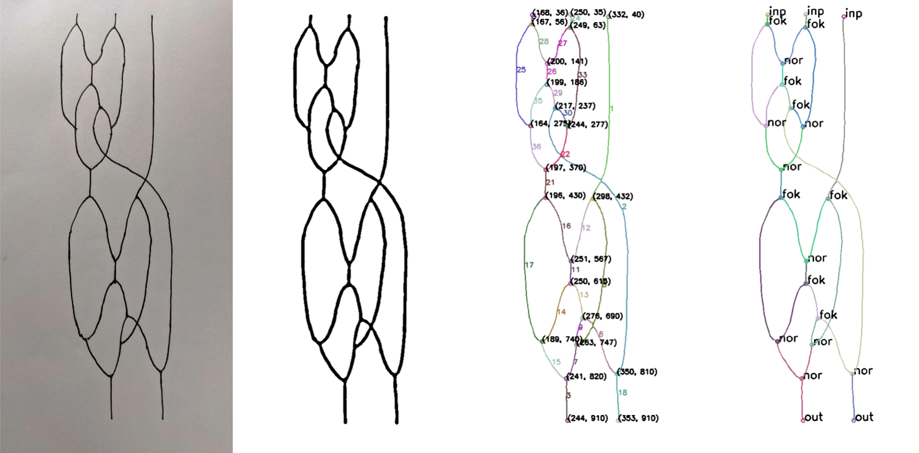
Adaptive threshold and morphological closing operator are applied to the input image to improve clarity. Then vector skeleton-tracing algorithm (coincidentally, also written by the author) is then used to extract the polylines. The endpoints of these polylines are analyzed to derive the nodes.
The resultant graph goes through a two-pass cleaning process, driven by a parameter "minimum edge length". First, tiny "stubs" (edges with one endpoint on a node, and the other floating) below this length, presumably coming from slight irregularities along the hand-drawn lines, are removed. Secondly, two nodes that are connected by edges below this length are merged into one node.
All nodes of degree other than three, are resolved as unconnected crossings, by the heuristic of least angle change, as mentioned before.
Note that the "minimum edge length" can be seen as the "resolution" of the detector, and drawer of Nor-Wires programs should seek to not introduce details below this size.
Finally, all the nodes are classified as "nor" or "fork", based on the orientation of incident wires. Similarly, all end points are classified as "input" or "output".
The execution of a Nor-Wires program can be animated in an interactive and asynchronous manner. The user would left click on a wire to "drop" a "dot" representing the one-signal, and right click on one to drop a dot representing the zero-signal. The signals would then travel through the wires carrying out any forking and NOR operations as they are encountered, producing more (or less) signals along the way. As a NOR node requires two inputs, once one input is received, the node would wait until the second signal arrives before applying the gate.
The animation can be overlain on the original hand-drawn graphics to enhance the illusion, which can be further improved if a projection-mapping and finger-tracking system is used.
Interacting with the animation is somewhat feels like watching the operation one of those marble-dropping machines.
Since as an isomorph of a Nor-Wires program is functionally equivalent to the original, the drawer has much freedom in terms of composition as well as quality of lines. They can distort or warp the program, use straight, curvy, shaky or wavy lines.
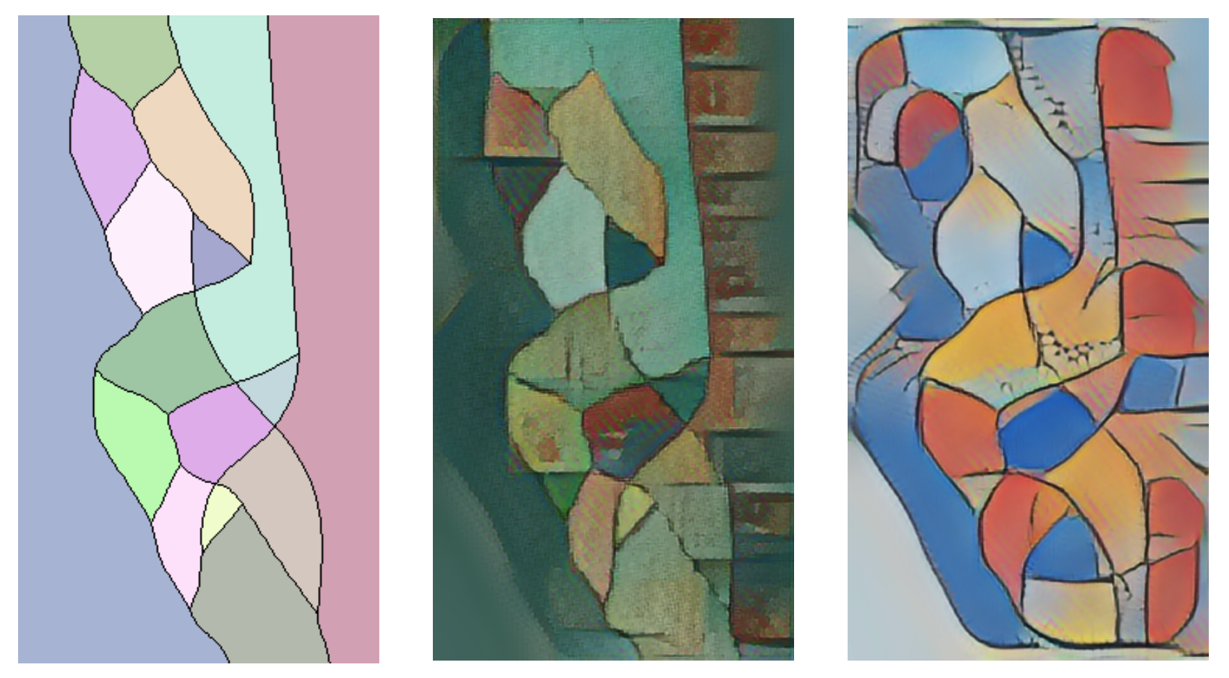
The spaces divided by the lines can also be colored freely, if it so pleases the drawer. Below is an example rendering of a program where each area is assigned a random color. It is somewhat reminiscent of the art of 20th century abstract painters, specifically that of Kandinsky and Joan Miró. As an experiment, style transfer is used to apply the style of these painters to the randomly colored program. Note that the style-transferred images are likely not reliably parsable with the computer vision algorithms described in the previous sections, as many extraneous lines and artifacts have been added by the neural net. (Nor do they reflect the artistic taste of the author of this thesis). They're chosen merely to give an idea of how a creative programmer might be able to paint their Nor-Wires program.
In Nor-Wires, NOR nodes and fork nodes are reflections of each other by the X-axis; so are input and output endpoints; Jumps are rotationally invariant. Therefore, an upside-down Nor-Wires program, is also a valid Nor-Wires program. All Nor-Wires programs can be viewed in two orientations: Nor-wire programs are ambigrammatic. However, what does the upside-down program do? How does it relate to the right-side up program?
The author implores the reader to turn this thesis (or alternatively, their head) upside-down, and have another look at each of the programs shown above (now below).
Nor-Wires succeeds in doing away with all symbols; Freehand lines are the only element; Meaning is derived from an inherent property of the drawing: topology. However, it can also be argued that Nor-Wires is essentially unmarked circuit diagrams, by utilizing the "loophole" that if all the gates are the same gate (universal NOR gate), they do not need to be distinguished from each other. It then inherits all the metaphors from circuit diagrams, such as signals and boolean algebra.
Is there other ways to design drawing-based languages that do not base on circuits, while fundamental attributes such as shapes, topology and spatial relationships further come into play? Stay tuned for the following sections.
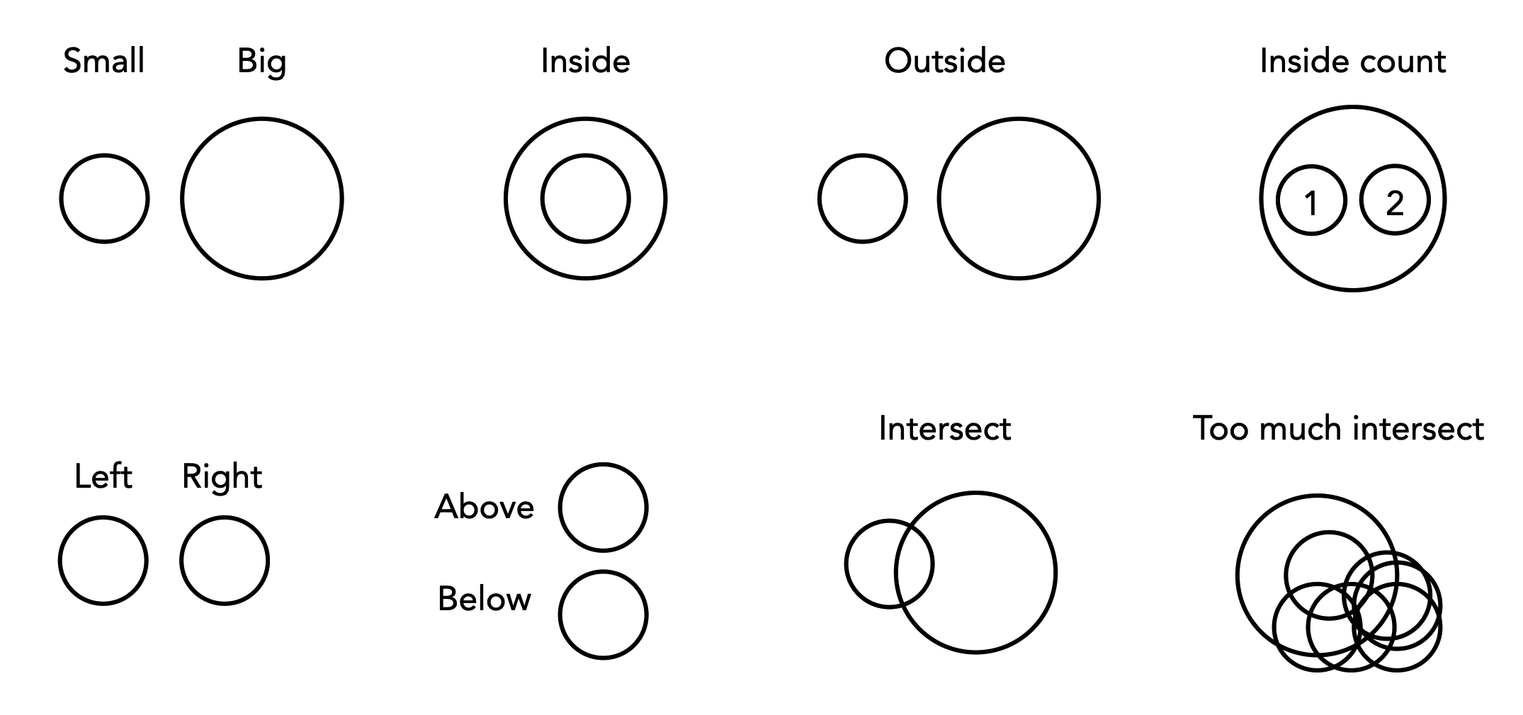
To find the true language of drawing, perhaps it is prudent to start with studying the basic elements of drawing, or the primitives. How can morphological properties and spatial interactions between primitives give rise to meaning? What would be the language of, say, circles? What would be the language of lines? What would be the language of points, of triangles, of polygons?
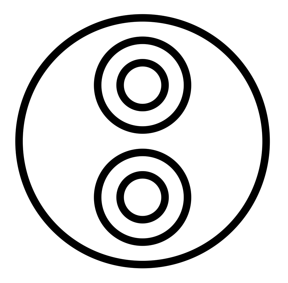
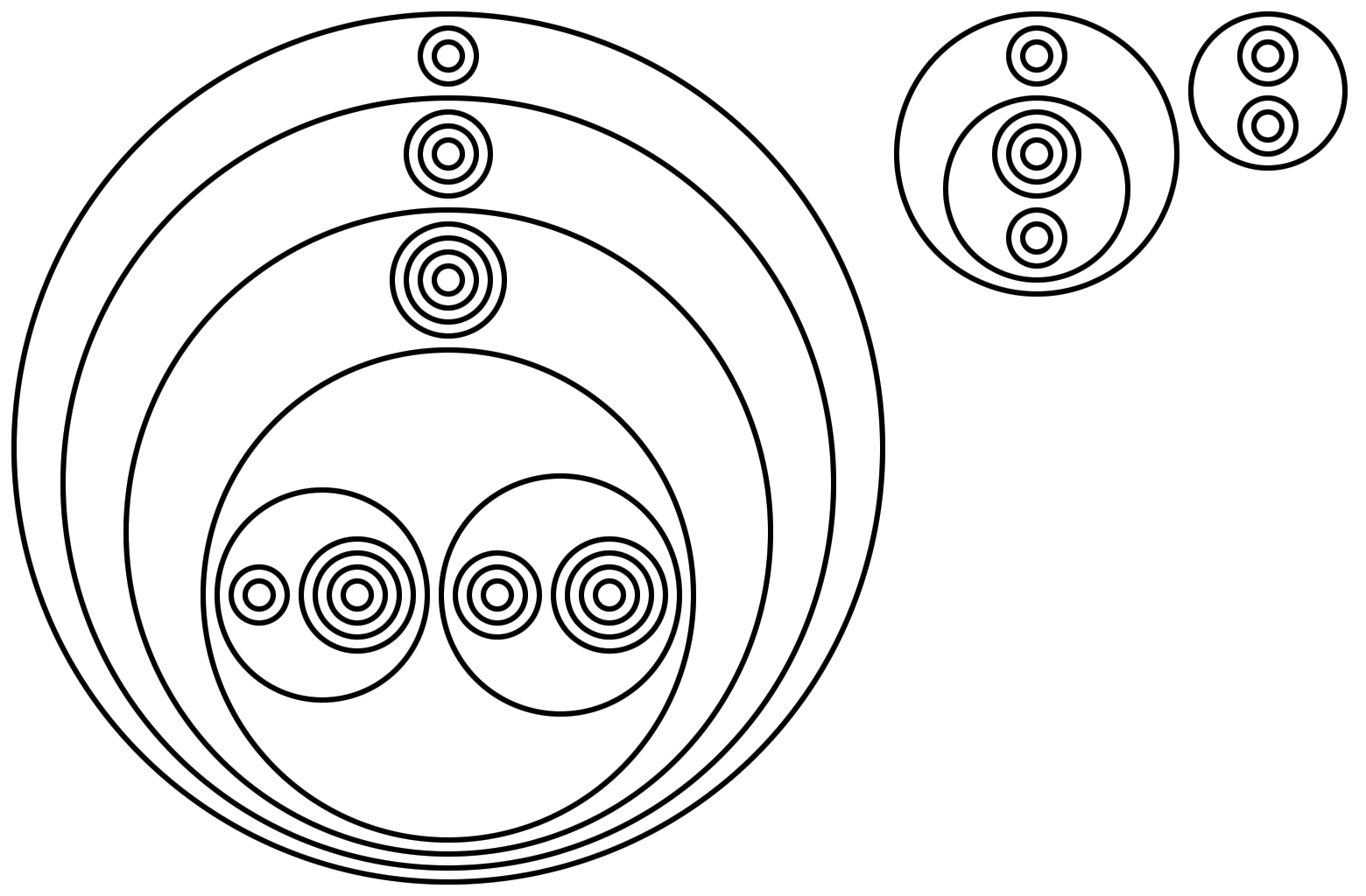
A circle is a collection of points of a certain distance away from a given center. Circles can be small, or they can be big. They can be inside, outside, to the left, right, above, below of other circles. They may intersect or tangent each other, or be very far away or right next to each other. They may not, however, be rotated, squashed, or sheared. Can these concepts be mapped to constructs in programming languages?
A (λ) language of circles is defined as follows:
To illustrate, here is λx.x, the identity function:
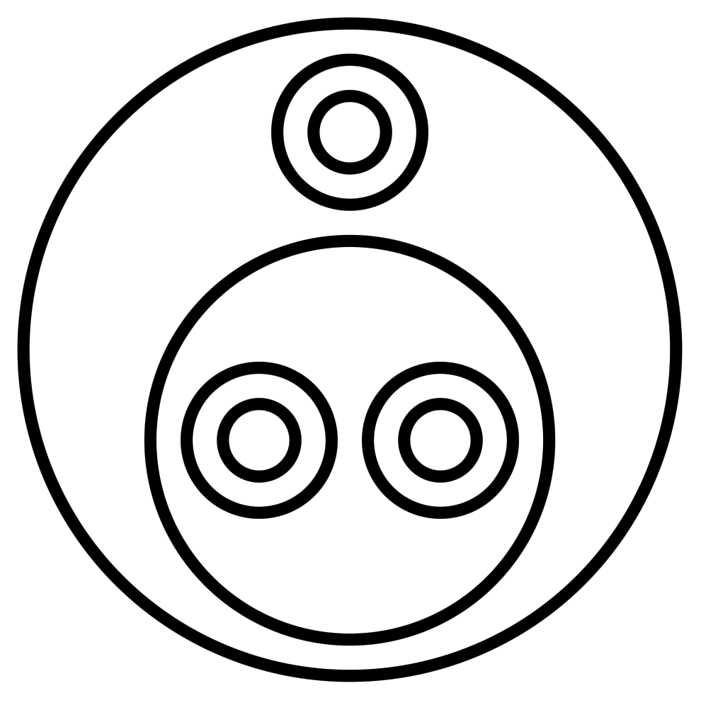
Here is a slightly more complex example, the little ω combinator (λx.x x), which applies the argument to itself:
We can use the ω combinator to define the Ω combinator (ω ω):
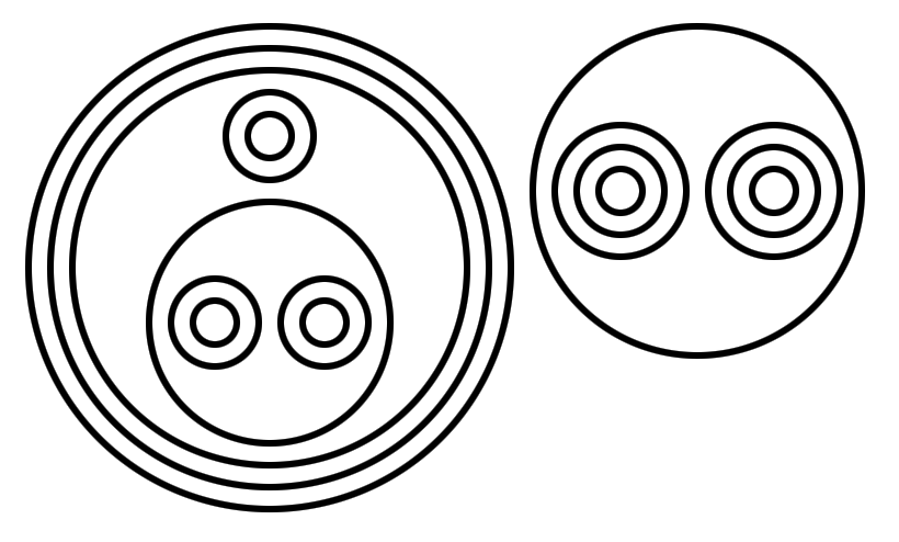
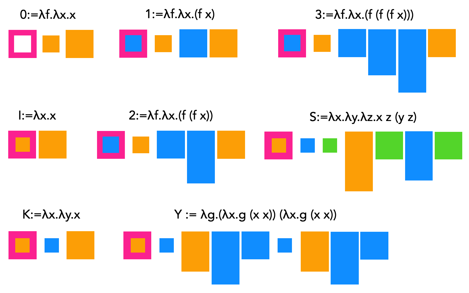
0 := λf.λx.x
1 := λf.λx.(f x)
2 := λf.λx.(f (f x))
3 := λf.λx.(f (f (f x)))
4 := λf.λx.(f (f (f (f x))))
...
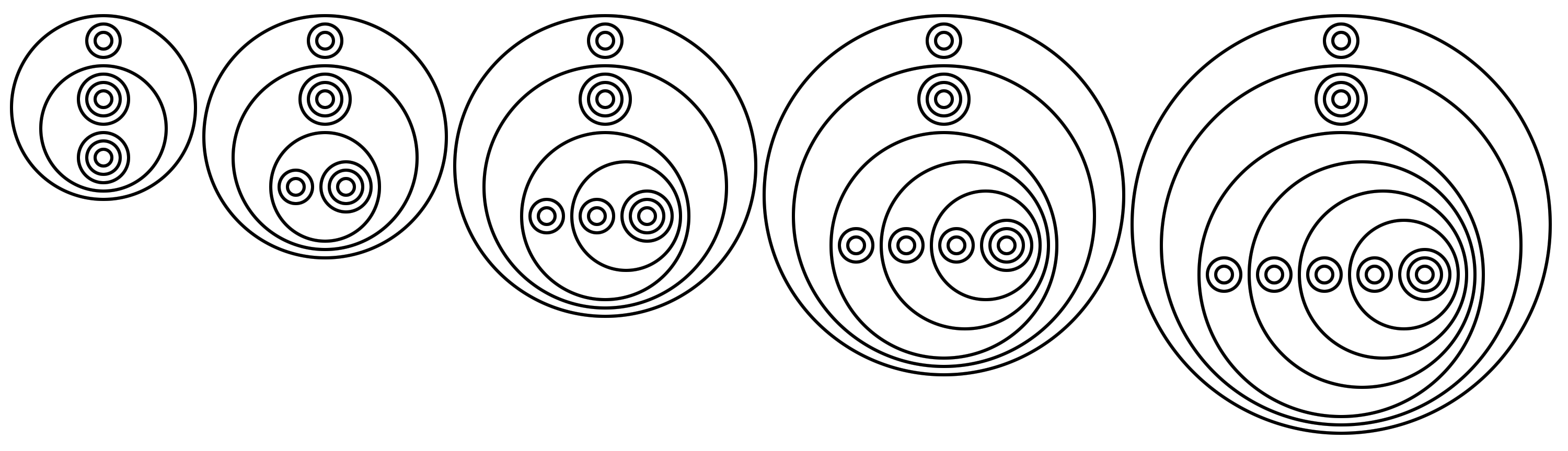
Similar to λ-2D, the language is also based on lambda calculus; But instead of having separate symbols for function definition and application, they're mapped to spatial arrangement of the circles. Instead of using wires to pass values, flow is derived from the structural hierarchy of enclosing circles. Because function definition and application both have "arity" of 2, the semantic meaning of concentric circles is free to be used as identifiers.
An aLoC program can also be conveniently represented using a string of ASCII text, which would be useful for transmission and storage.
The text notation has an alphabet of three characters: left parenthesis "(", right parenthesis ")" and newline "\n", as detailed in the Backus-Naur form (BNF) below:
<circ> ::= "(" (<circ> "\n"? <circ>)? ")"
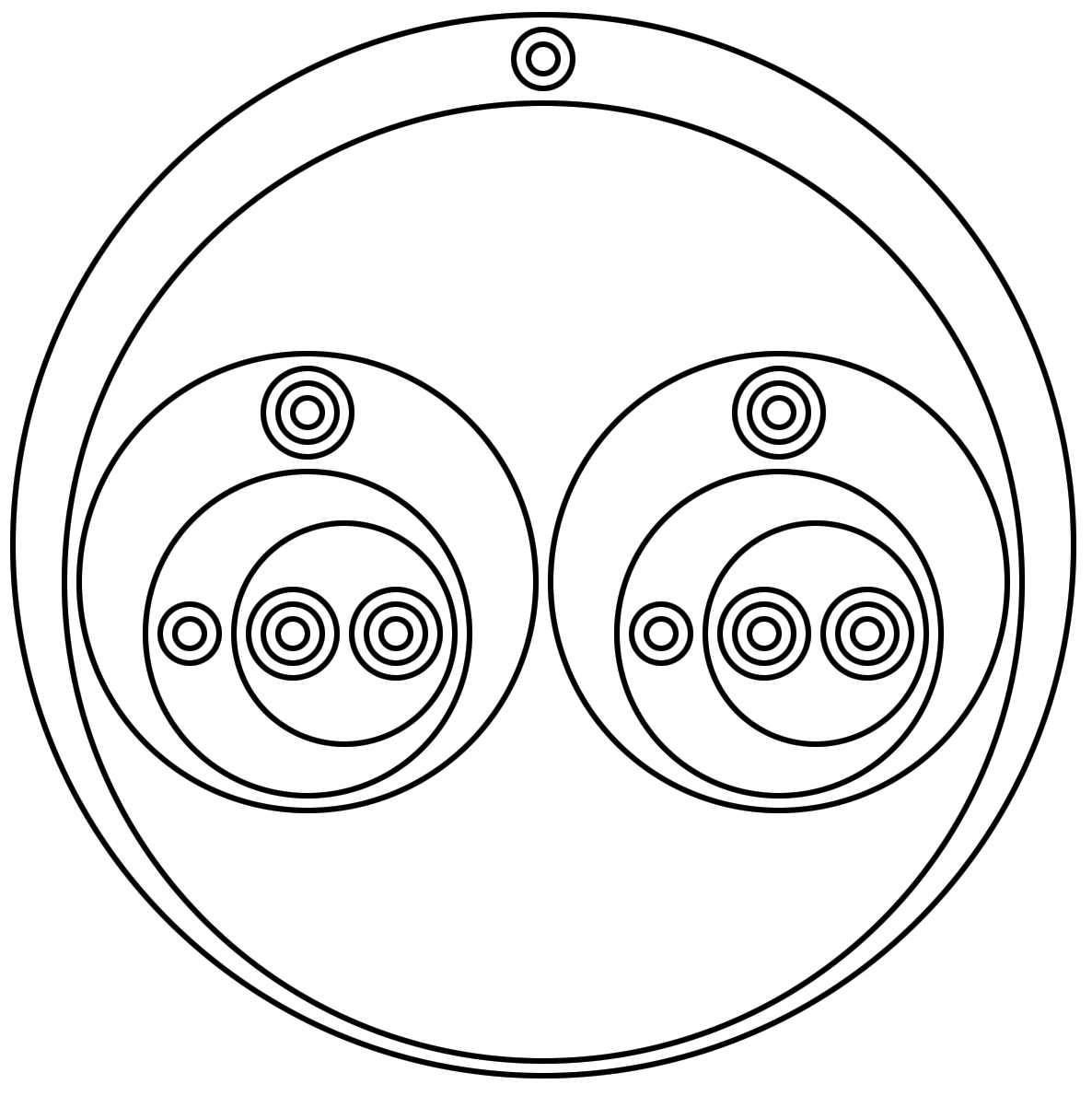
Basically, a circle is represented as a pair of parentheses "()". A function application is written as "(()())", while a function definition is written as "(()\n())". The Y-combinator shown previously can therefore be encoded as:
((())
((((()))
((())(((()))((())))))(((()))
((())(((()))((())))))))
Looks even more confusing, I know.
A simple algorithm for compiling aLoC programs to and from lambda calculus is described.
We make use of an abstract syntax tree as an intermediate format for the conversion, defined recursively as follows:
Node = DEFN(ARG:Node, RET:Node)
     | CALL(FUN:Node, ARG:Node)
     | IDEN(Num)
Num  = 1 | 2 | 3 | 4 | ...
Which can be trivially translated to and from the canonical way of expressing lambda calculus. For example, the ω combinator (λx.x x) can be represented as follows:
DEFN(
	ARG:IDEN(1)
	RET:CALL(
		FUN:IDEN(1)
		ARG:IDEN(1)
	)
)
Then, a routine to generate an aLoC program from the AST can be implemented as follows:
function GENERATE(e)
	case e of
	  IDEN(n):
			o := {}
			for i in 0...n
				o = o + CIRCLE(x:0, y:0, r:i+1)
			return o
	| DEFN(ARG:a,RET:r):
			p := GENERATE(a)
			q := GENERATE(r)
			u := p[LAST]
			v := q[LAST]
			return p + TRANSLATE(q, u.x-v.x,
			                        (u.y+u.r+v.r+1)-v.y) +
			           CIRCLE(x:u.x, y:u.y+v.r+0.5, r:u.r+v.r+1.5)
	| CALL(FUN:f,ARG:a):
			p := GENERATE(f)
			q := GENERATE(a)
			u := p[LAST]
			v := q[LAST]
			return p + TRANSLATE(q, (u.x+u.r+v.r+1)-v.x,
			                        u.y-v.y) +
			           CIRCLE(x:u.x+v.r+0.5,
			                  y:u.y,
			                  r:(u.r+v.r)+1.5)
end
The routine returns an array of circles as tuples (x-coordinate, y-coordinate, radius), where the smallest circle will have a radius of 1. The programmer can apply further normalization to the coordinates to fit the program into a desirable viewport. The Circles program examples shown in the previous section are generated using this routine.
Reversely, a routine to de-compile an array of circles back to a lambda expression may be implemented as follows:
function DEGENERATE(c: circle)
	while c has exactly one child do
		c.children := c.children[0].children
		if c does not have an ID then c.ID = 0
		c.ID := c.ID + 1
	end
	if c has no children then
		return IDEN(c.ID)
	end
	if c has exactly two children (a,b) then
		p := DEGENERATE(a)
		q := DEGENERATE(b)
		if ABS(a.x-b.x) > ABS(a.y-b.y) then
			return CALL(FUN:p,ARG:q)
		else
			return DEFN(arg:p,RET:q)
		end
	end
end

C : list<circle> = {...}
SORT(C, RADIUS, INCREAS\ING_ORDER)
for i in 0...LEN(C) do
	for j in (i+1)...LEN(C) do
		if C[i] is inside C[j] then
			C[j].children += C[i]
			C[i].parent = C[j]
			break
		end
	end
end

O : list<Node> = {}
for each c in C which has no parent do
	O = O + DEGENERATE(c)
end
aLoC programs can take up much space as they become more complex. Since the semantics of aLoC programs only depend on inter-circle relationships, it is possible to deform the circles as long as these relationships are kept. Therefore, the drawer has much freedom in expression when drawing an aLoC program; This is similar to Nor-wires.
Based on these considerations, a physics simulator was developed to "shrink" aLoC programs in an organic manner for better space utilization and a new aesthetic. Below as an example output:
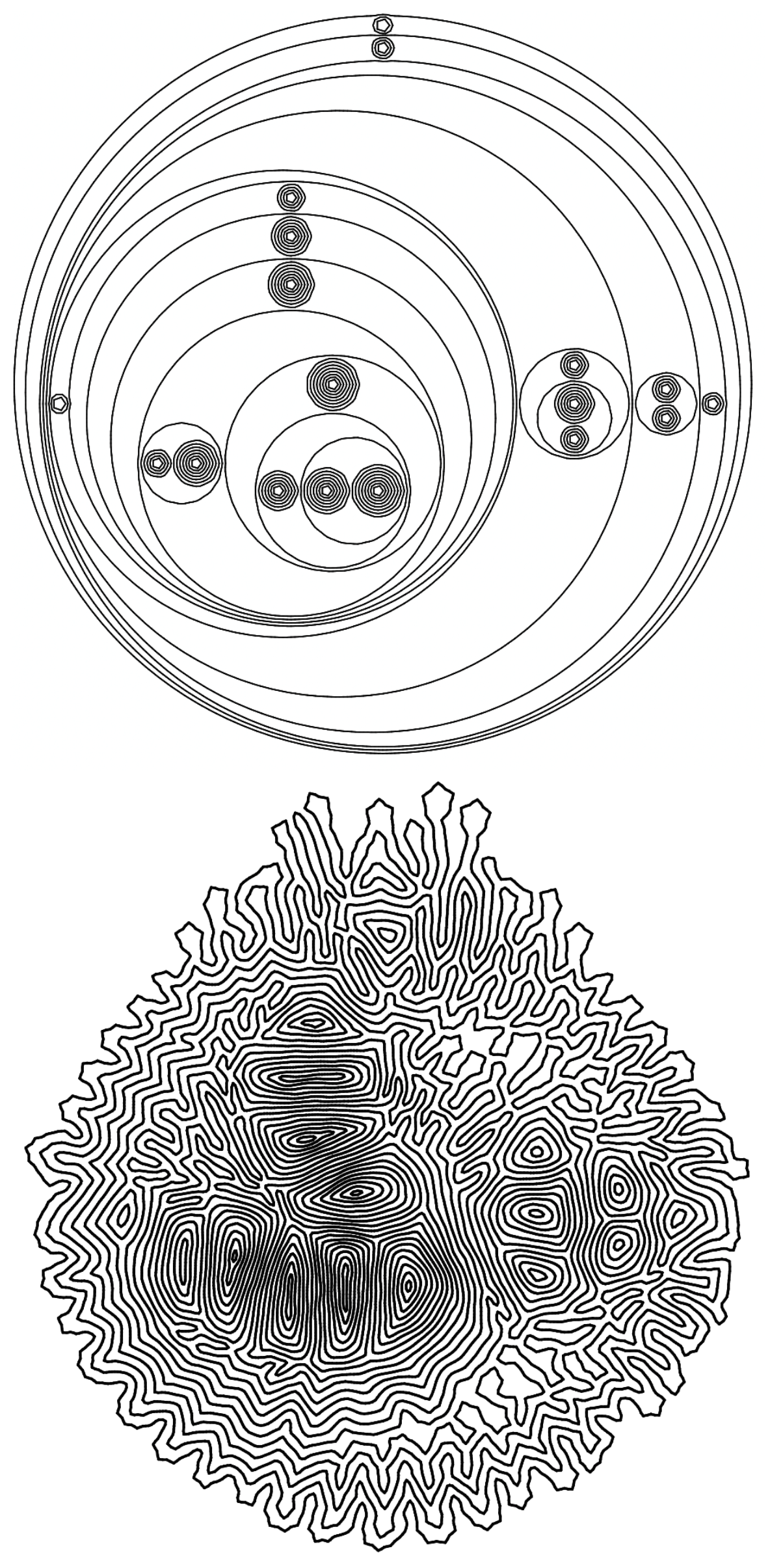
Parameters such of strength of various forces can be tweaked to create different results.
The details for this simulator will be discussed later in this thesis rather than here, for it functionally is a subset of the simulator for the next programming language that is about to be introduced: A Language of Lines.
When the dots are so close to one another that they cannot be individually recognized, the sensation of direction is increased, and the chain of dots becomes another distinctive visual element, a line.
― Donis A. Dondis, A Primer of Visual Literacy
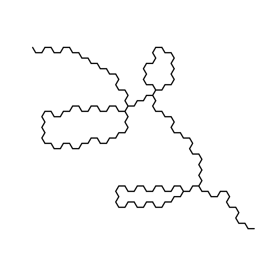
Similar to aLoC, the conception of a Language of Lines (aLoL, not to be confused with LOL) started with an analysis of morphological properties and spatial interactions between the primitives.
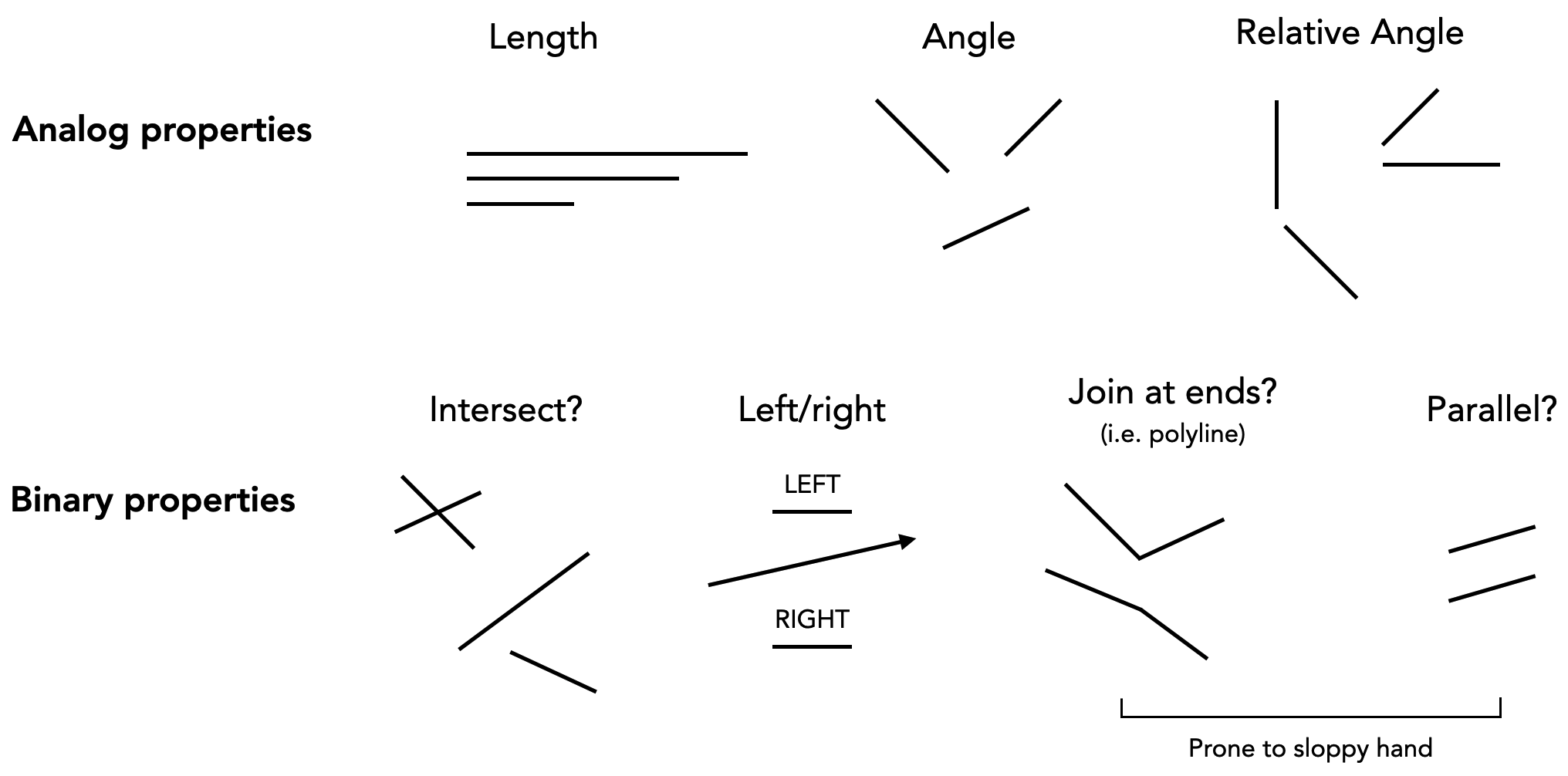
A (λ) language of lines is defined as follows:
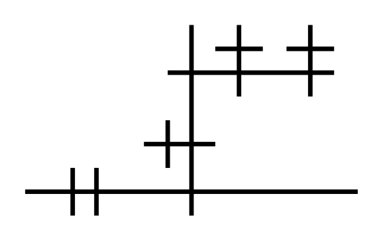
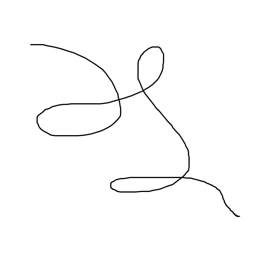
Where D/REF stands for definition/reference. Though these rules have a lot of words, it is quite intuitive in practice. For example, to define the identity function (λx.x), we can draw:
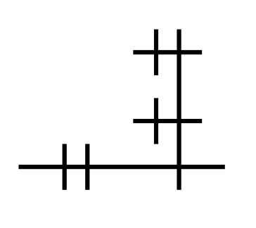
Next, let's look at something slightly more complex, the little ω combinator (λx.x x), which applies the argument to itself:
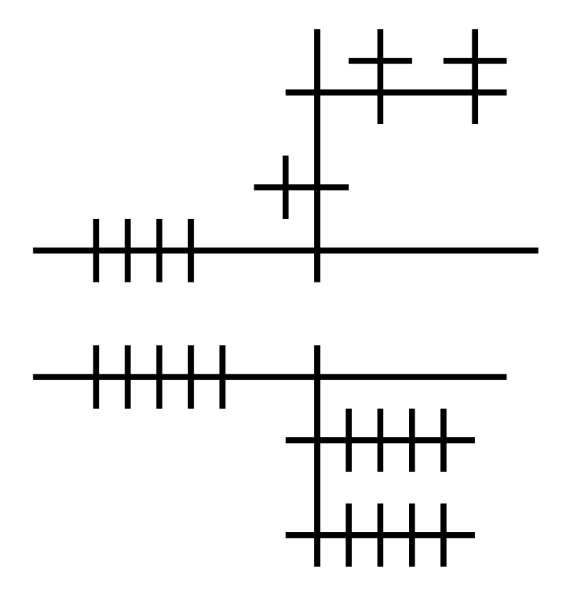
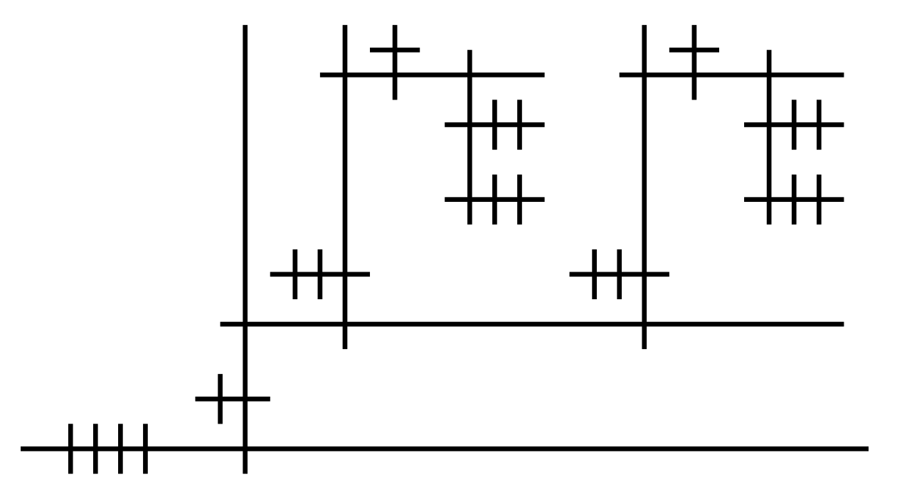
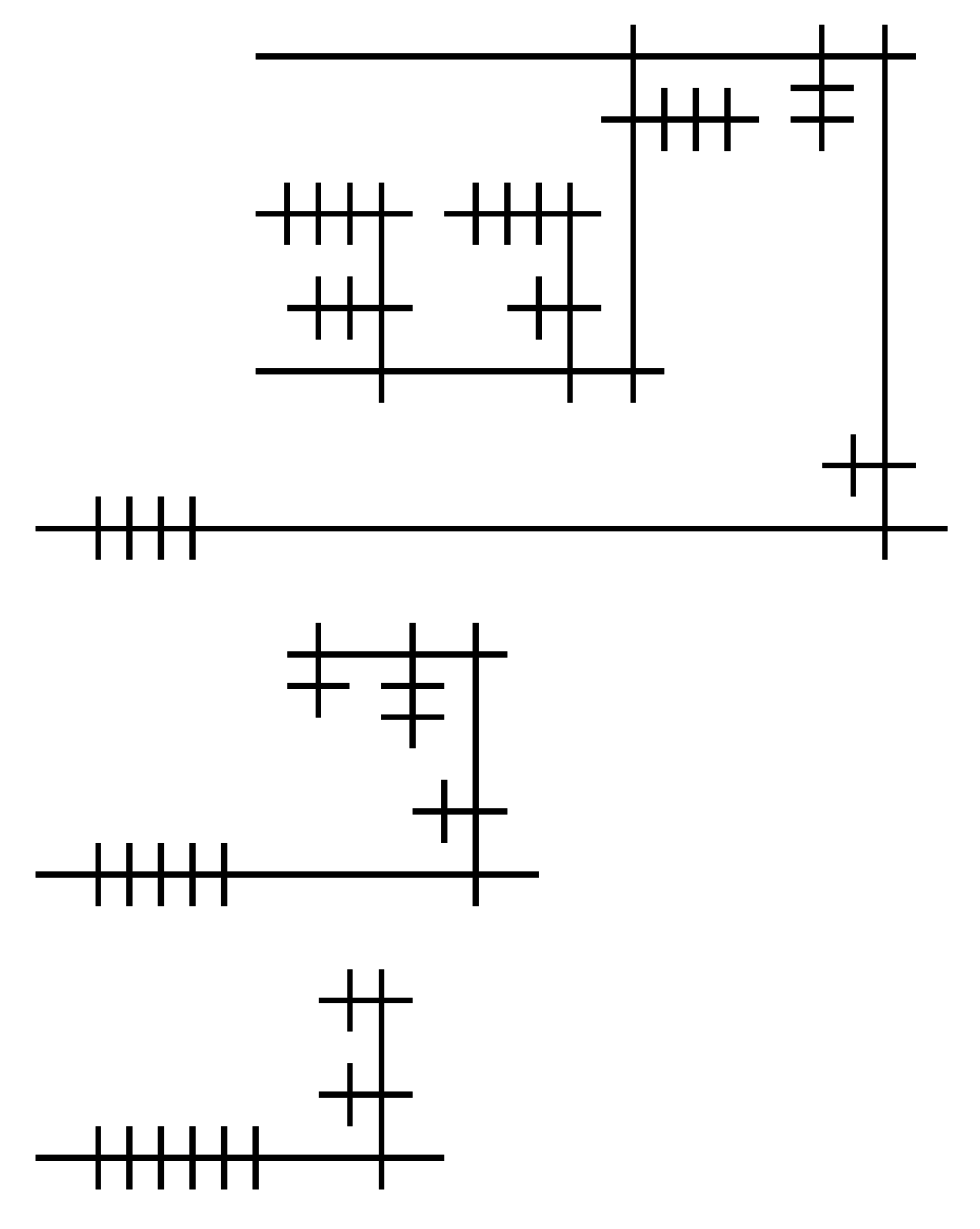
Similar to aLoC, aLoL is based on lambda calculus; But instead of mapping the duality of function definition and application to vertical and horizontal layout of circles, they are mapped to the left/right-hand sides of a direction.
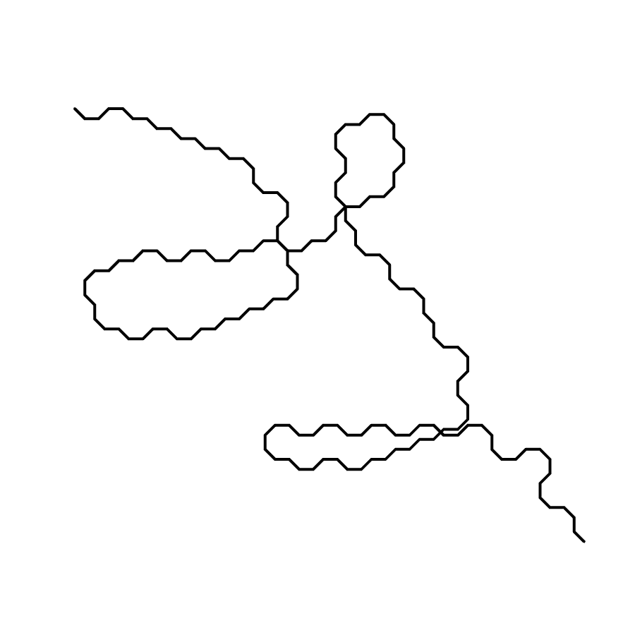
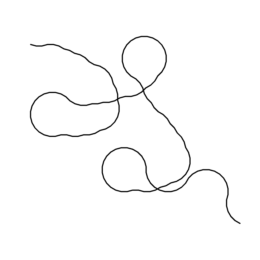
Though the examples above are drawn with axis-aligned lines, it is not imperative to do so. Slanted lines, curved lines, and even wiggly lines would also work, as long as the intersections are kept. This will be further demonstrated in later sections. Like in Nor-wires and aLoC, it leaves room for sloppiness and artistic expression.
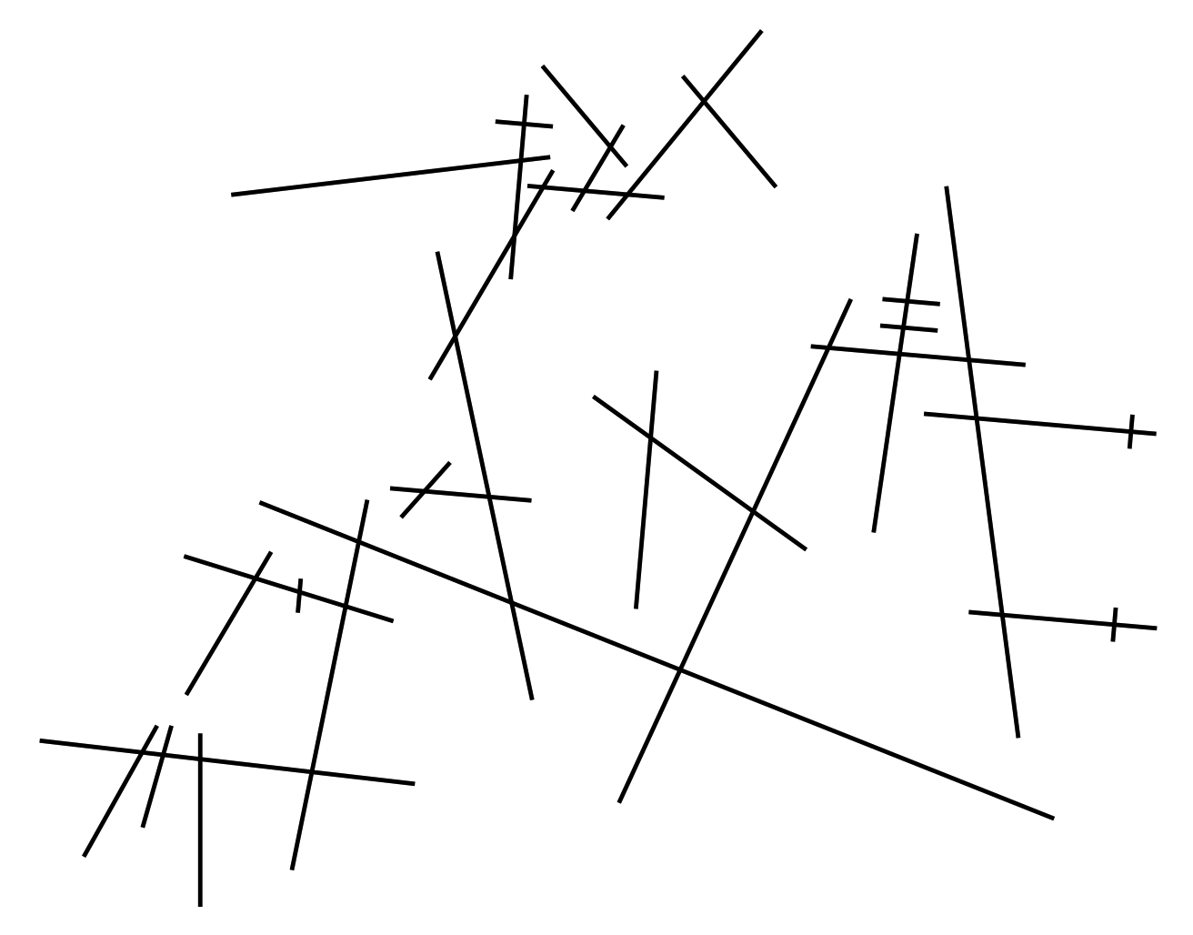
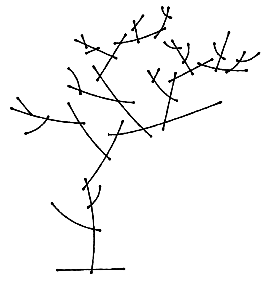
As you can see above, aLoL programs can be easily hidden in inconspicuous nature drawings.
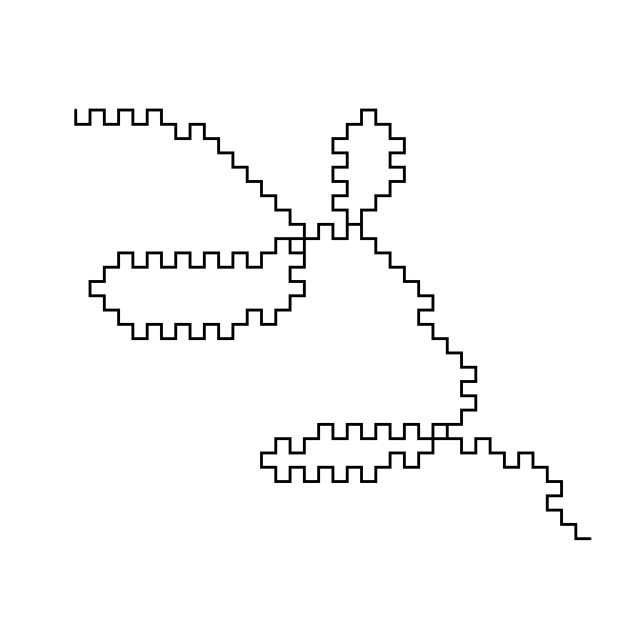
If the rectilinear style is preferred however, aLoL programs can be drawn with ASCII characters, or unicode box-drawing characters (U+2500 - U+257F), which might facilitate transmission and storage.
       +
      ++-+     +
    +++  +++  ++-+
      |  |  +++  +++
      |  +++  |  |
    +-+-------+  +++
   ++
+++-+
The algorithm for compiling aLoL programs to and from lambda calculus is rather similar to those for aLoC (see previous section). Nevertheless, a few techniques might worth additional mentioning.
First, the recursive generation of aLoL programs should use a bottom-up approach. That is, the parent node in the recursion tree does not start generating, until all its child nodes returned generation results. This is due to the fact that the parent node doesn't have information about how much space the child would cover, and if the parent node is generated first, the child node would need to be scaled down to fit, whose child would also be scaled down in turn, thus creating fractal-like forms with legibility issues toward the recursive bottom (and vast empty spaces toward the recursive top).
Additionally, a grid-based system is used. Each grid is one of: an intersection (+), a vertical bar (|), a horizontal bar (-), or empty sapce. However, when generating the segments, they need not be broken up to fit into the grids: the grids are merely for facilitating alignment and calculation of bounding areas.
This baseline implementation, for simplicity, uses the bounding boxes of child nodes to plan space, even though the bounding box might be barely filled. This creates quite a bit of inefficiency in space usage. One possible improvement is to implement a more sophisticated "collision detection" scheme, accurate to each aforementioned grid-cell, greedily squeezing subgraphs into unused spaces.
In the following section, an alternative approach based on physics simulation, is introduced, which also produces a more organic and painterly aesthetic.
As the requirements for this simulation is quite peculiar (as detailed below), a dedicated, custom physics system is written from scratch, instead of being reliant on popular physics libraries or frameworks.
The system is mostly based on spring simulation, where each node is connected to its neighbors via tiny springs following Hooke's Law (F=-kx). Then, a centripetal force is introduced, to make the graph "shrink" toward the center. However, there are a few twists:
If the physics scene is built only once at the beginning of the simulation, the lines, instead of being continuously shrunk, will start to make "folds" and "wiggles". This is because a "rope" made of a series of springs would have a "natural" length, and could not become much shorter than that. While this could also produce an interesting look, it runs counter to our sub-goal of optimizing for space.
Therefore, the trick is that, every few iterations, the physics scene should be rebuilt from scratch, by resampling all the edges in the graph. This way, once the shrinkable springs have shrunk their due amount, they're replaced by new springs which have shorter natural length, so they can shrink even more in the upcoming iterations. The "unshrinkable" springs (those that cannot shrink anymore, due to pull by other forces), on the other hand, would be replaced by new springs of equal (or even greater) length, and therefore functionally unaffected.
In addition to spring tension, a few other forces are introduced for our particular case. First, under no circumstances should a new intersection be introduced, as this would alter the meaning of the program, and is the worst situation possible. Therefore, nodes should try their best to repel anything that is not their neighbor, including both other nodes as well as edges. To further ensure unwanted intersections absolutely do not happen, after each batch of iterations, the system will do a "fatal error check", if it finds a new intersection, the simulation will be "time-warped" to the previous state, and every node is given a small random jitter (to break deterministic future), and the iteration will be retried.
All nodes that have four incident edges (i.e. intersection points) should also try to ensure that these four edges make roughly 90° angles with each other, and their order is absolutely never changed. If the four edges "collapse" into small angles, the intersection becomes illegible; If the order is changed, the meaning of the program changes.
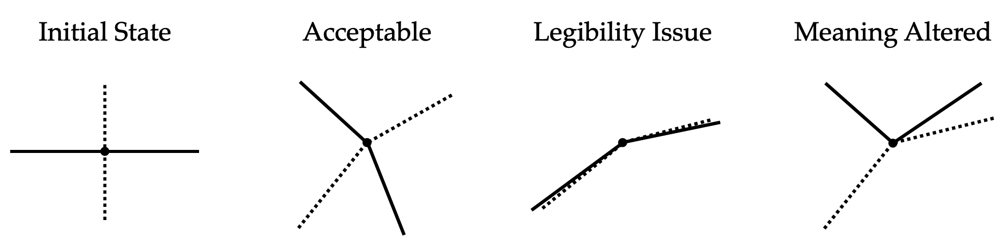
Other nodes, which usually have two incident edges (except endpoints), should also make a small effort to keep the edges at 180° angles from one another, this is to make the curves look smooth(-ish), and is therefore a less imperative constraint.
Heun's method (2nd order Runge-Kutta) is used for the numerical integration in this implementation, though higher-order ones can be upgraded to.
Spatial hashing (dividing the scene into conveniently-sized grids) is used to speed up distance queries. This could also be easily upgraded to KD-trees.
Following is the pseudo code for the main spring simulation:
function SIMULATE_SPRINGS(nodes, dt, flags)
	for each k in nodes do
		k.v := k.v * damping
		k.a := 0
	if flags & FORCE_TENSION then
		for each k in nodes do
			for each n in k.neighbors do
				d := n - k
				l := ||d||
				d := d / l
				k.a := k.a + (l-1) * d * factor
	if flags & FORCE_TORQUE then
		for each k in nodes do
			n := count(n.neighbors)
			if n != 4 then continue
			for i in 0...n do
				p := k.neighbors[i]
				q := k.neighbors[(i+1)%n]
				d := angle_diff(p,q)-PI/2
				u := {d*(k.y-p.y), d*(p.x-k.x)}
				v := {d*(k.y-q.y), d*(q.x-k.x)}
				p.a := p.a + u * factor;
				q.a := q.a - v * factor;
	if flags & FORCE_STRAIGHTEN then
		for each k in nodes do
			n := count(n.neighbors)
			if n != 2 then continue
			p := k.neighbors[0]
			q := k.neighbors[1]
			...
			(apply torque, like previous case)
	if flags & FORCE_REPEL then
		for each k in nodes do
			N := query_by_dist(nodes, 1)
			for each n in N do
				if k is n then continue
				if k.neighbors include n then continue
				d := n - k
				l := ||d||
				d := d / l
				k.a := k.a + (l-1)*d * factor;
		for each k in nodes do
			z := 1
			if count(k.neighbors) == 4 then
				z := 0
				for each n in n.neighbors do
					z := z + dist(n,k)
			N := query_by_dist(nodes, 3)
			for each n in N do
				for each m in n.neighbors do
					d := point_to_segment(k,n,m)
					l := ||d||
					d := d / l
					k.a := k.a + (l-1)*d*z *factor
					m.a := m.a + (1-l)*d/z *factor
					n.a := n.a + (1-l)*d/z *factor
	if flags & FORCE_CENTRIPETAL then
		c := centroid(nodes)
		for each k in nodes do
			d := c - k
			l := ||d||
			k.a := k.a + l*l*d*factor;

	HEUNS_METHOD_INTEGRATE(nodes, dt)
end
To drive the physics system, the spring simulation is run in a nested loop. In the outer loop, the graph is first simplified (greedily removing nodes, whom, if removed, neither introduce nor reduce intersections), and then resampled (edges are split up until they're shorter than a given length). Next, a few iterations of spring simulation is run. The aforementioned fatal error checking procedure is then applied, before starting the next outer iteration.
Prior to outputting the final result, a few more iterations of spring simulation is run, though without the centripetal force. This is to refine the result and smooth out any small disturbances.
nodes := {...}
for i in 0...40 do
	nodes' := deep_copy(nodes)
	SIMPLIFY_NODES(nodes)
	RESAMPLE_NODES(nodes)
	for j in 0...20 do
		SIMULATE_SPRINGS(nodes, 0.1*(1-j/100), 0xffff)
	if FATAL_CHECK(nodes) == FAILED then
		nodes := nodes'
		for each k in nodes do
			k.x := k.x + random(-EPSILON,EPSILON)
			k.y := k.y + random(-EPSILON,EPSILON)
RESAMPLE_NODES(nodes)
for in 0...3 do
	SIMULATE_SPRINGS(nodes, 0.05,
		FORCE_REPEL|FORCE_STRAIGHT|FORCE_TORQUE)
READOUT()
Here is the example result on the fibonacci program (λn.λf.n(λc.λa.λb.c b(λx.a (b x)))(λx.λy.x)(λx.x)f):
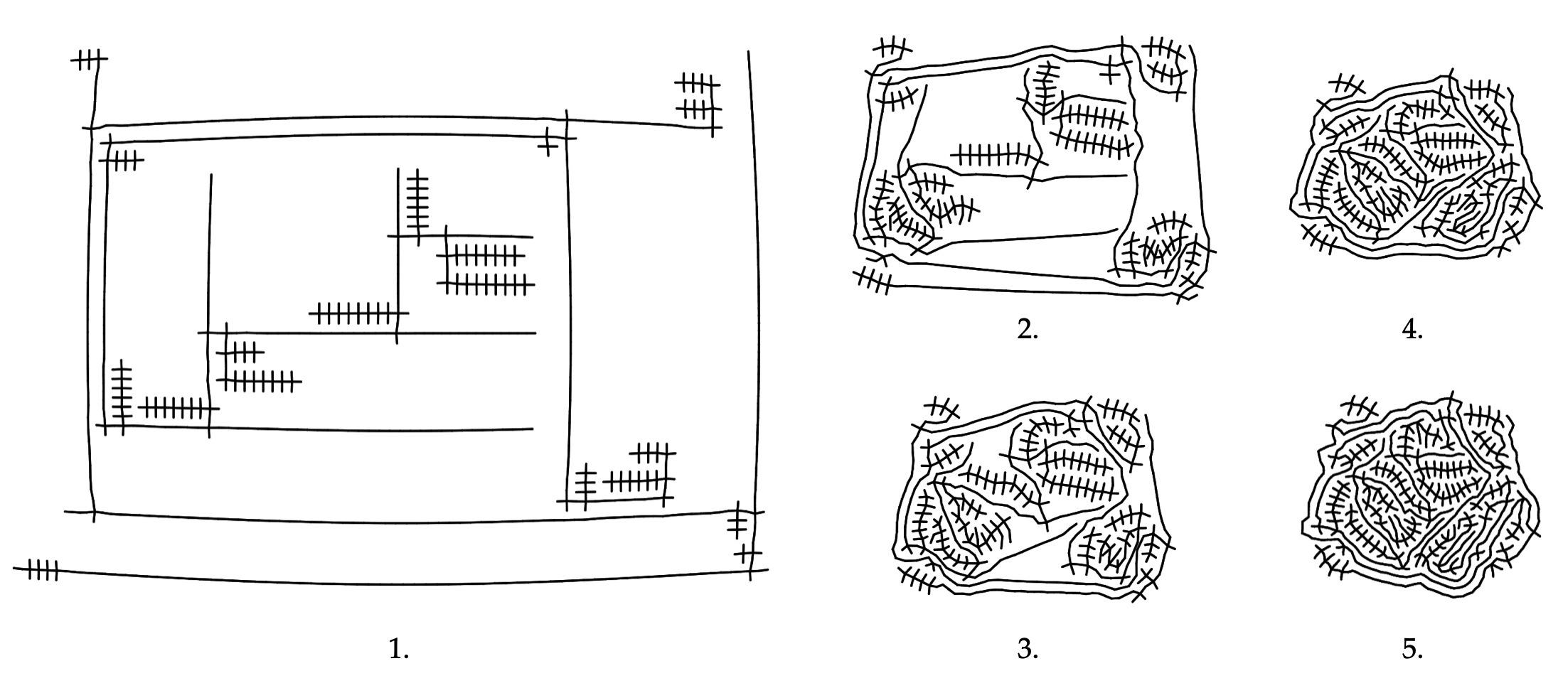
As you can see, the final result occupies less than ⅕ of the original size.
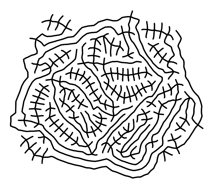
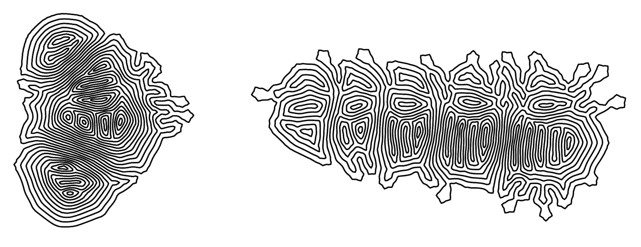
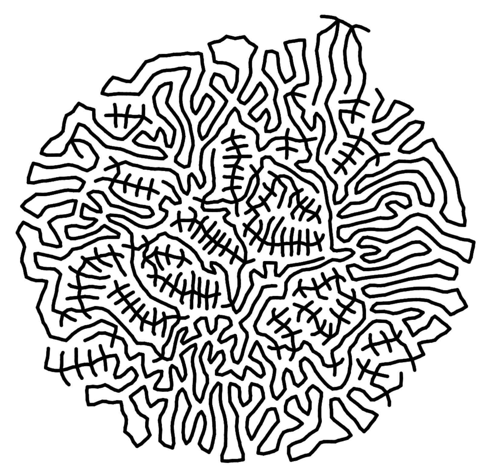
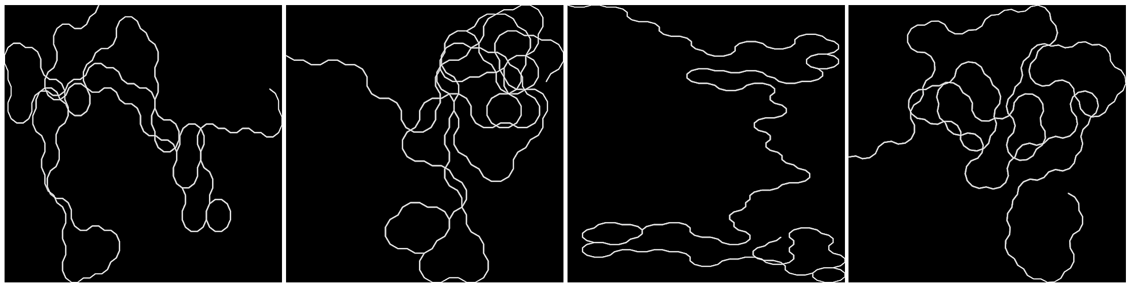
Post-processing can be further applied to the output of the physics simulation, to provide more opportunities for stylistic choices. Below you can see two such examples. On the left, distance transform is computed for the image, and simple Lambertian shading is added to give an illusion of volume. (This is in response to a comment that these programs look like stitches on wounds).
The right image is achieved using Lloyd's relaxation on Voronoi diagrams. The algorithm tries to place each site at the center of its cell, iteratively, such that in the end, the vertices are spread out most evenly over the space.
The algorithm was initially used in place of the physics simulation, due to the author's loathing of explosions. However, it did not work then, as the algorithm has no control over the behavior of the original edges. After the simulation is done however, the drawing is already well-packed, and running Lloyd's relaxation no longer turns it into a big yarn of mess. Instead, a ton of interesting (though harmless) wiggles are introduced, serving as a reminder that, spreading out vertices of a drawing evenly, is not equivalent to spreading out a drawing evenly (whatever that means).
As the computer vision techniques for parsing aLoC and aLoL programs from pen-on-paper drawings would be very similar to those used for Nor-Wires (adaptive threshold → polyline extraction → graph reconstruction), they are omitted here.
Since both aLoC/aLoL and λ-2D are based on lambda calculus, it is not too massive an undertaking to make a transpiler capable of converting a reasonable subset of the latter to the former. As λ-2D is considerably higher level, this would enable us to see what aLoC/aLoL programs really look like at a larger scale, without having to spend days constructing all the trivial parts in lambda calculus (however fun that may be).
In this implementation, the general strategy is to use Church encoding for natural numbers, and cons-cell lists for λ-2D bitmaps. Support for signed and floating point number are omitted for the sake of simplicity. Overheads are also to be expected compared to hand-crafted programs, as is common in such processes. Still, many interesting programs can be constructed under these limitations.
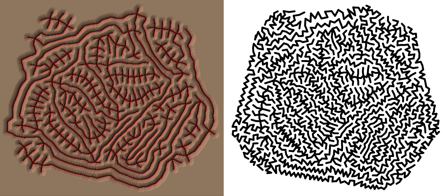
Below is the Bresenham's line algorithm in aLoC (automatically translated from a λ-2D implementation shown, albeit partially, earlier).
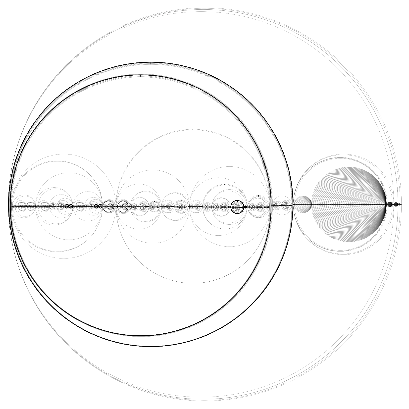
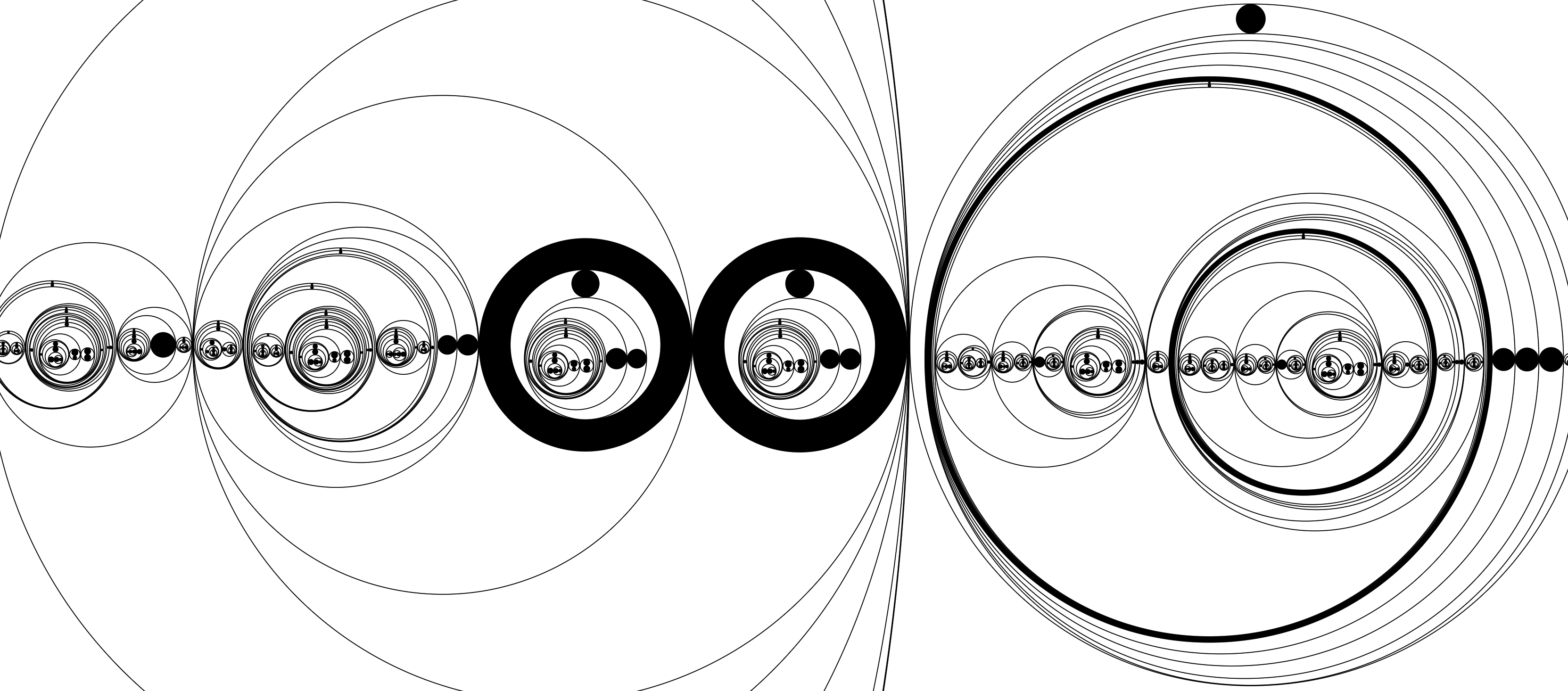
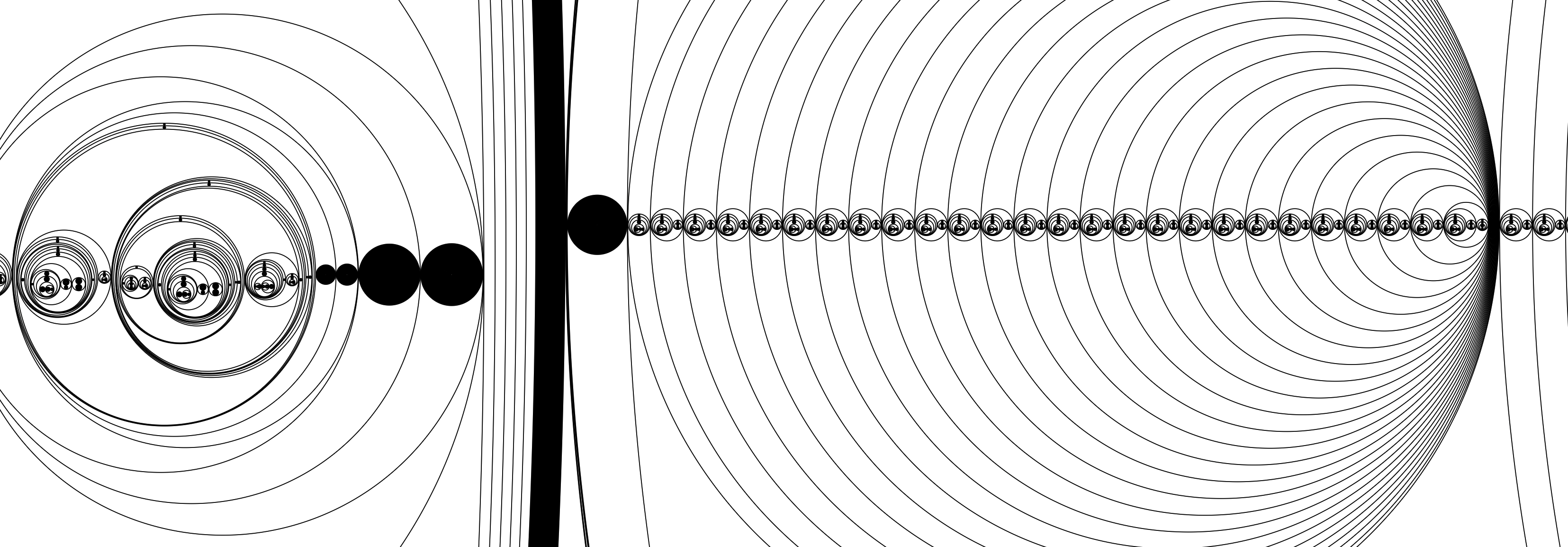
The program consists of 21,594 circles, and exhibits fractal-like patterns. Zooming in and panning around, it feels not unlike looking at the Mandelbrot set.
A Language of Circles keeps track of ID's by counting rings of concentric circles. This causes the size of the program to increase at a super-linear speed, every time a new variable is introduced. It might also create issues for automatic detection algorithms, as many rings of concentric circles would look like one ring with thick, gray, stroke under low resolution. In this respect, A Language of Lines is much more optimized, as only a very small tick needs to be added for each new ID. However, as the count gets large, it would still start to look confusing. Perhaps such is the woe of being stuck to a unary number system.
In addition to aLoC and aLoL, more languages of primitives can be designed in a similar way; In fact, there're also many alternative ways aLoC and aLoL could have been designed. However, for the sake of this thesis, these two representative examples are perhaps sufficient in illustrating the methodology used behind the category.
The languages of primitives succeed in creating visually-interesting and fully-functioning systems while using only a single type of primitive. They also permit much creative freedom for their drawers, allowing them to "hide" programs in "art". But it is also arguable, that they're merely forms of "diagrams" for expressing lambda calculus. Or perhaps, they can also be called alternative "visualizations" thereof. However, I believe the most interesting aspect is the methodology: How can one map geometries into semantics? How to study the primitive shapes, and explore the way with which their properties can be used to express programming constructs?
Perhaps it can be said, that the association with lambda calculus is incidental; Given any computational system, there could be a language of circles and a language of lines made for it, using the process described in this chapter. Though undeniably, the inherent minimalism in lambda calculus made it an especially attractive option.
While λ-2D, Nor-Wires and the Languages of Primitives are fully-qualified programming languages, this chapter describes some drawing tools that, while not necessarily Turing-complete (some of them still are), nevertheless explores "programming-like" aspects of drawing, where some form of input, when structured in some meaningful way, would produce some non-random output, in however expected or unexpected fashion.
While minimalistic in nature, these "non-languages" aim to provoke novel ways of thinking about programming and drawing, and could perhaps be integrated as part of larger programming- or drawing-based tools and tool kits.
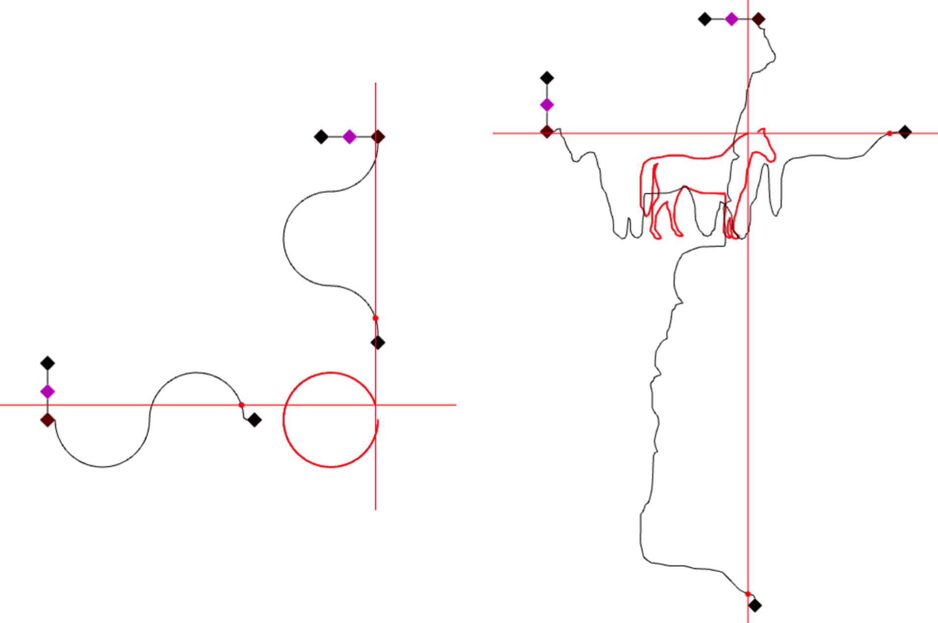
A line (or, more specifically, a curve, or polyline) can be used to encode a binary string, which can then be used to present computational concepts such as programs and data.
One straightforward way to achieve this is by encoding the line as a series of angle changes: if the line turns left at a certain point, it represents a zero; right, then one. For example, if a line turns left, then right, then right, then left again, it encodes the binary string 0110.
However, it can be somewhat difficult to see how many points there are in a continuous, hand-drawn line ― and which direction at each point is the line turning, if the angle is small.
Therefore we propose an "augmentation" of lines for such purposes ― a "resampling" algorithm to "normalize" both the angle and the segment length of a given polyline.
A naïve algorithm would simply take all the segments in the line, set each to the given length, and round its angle to the nearest value for "left" and "right". However, this would cause the new line to no longer resemble the old line, as the errors would accumulate.
Below is the pseudo-code for an improved algorithm, which compensates for error accumulation. Additionally, it allows snapping to an arbitrary list of "allowed angles".
let as = [-PI/4,PI/4]; // allowed angles
let lookahead = 5;     // window size
let d = 10;            // segment length
function make(ps,rs,n0){
	if (n0 >= ps.length){
		return rs;
	}
	let [x0,y0] = rs[rs.length-1];
	let a0 = 0;
	if (rs.length >= 2){
		a0 = atan2(y0-rs[rs.length-2][1],x0-rs[rs.length-2][0]);
	}
	let pp = ps.slice(n0,n0+lookahead);
	let md = Infinity;
	let mn = n0;
	let mr = [];
	for (let i = 0; i < as.length; i++){
		let x1 = x0 + cos(a0-as[i])*d;
		let y1 = y0 + sin(a0-as[i])*d;
		let [i1,d1] = pt_dist_pline([x1,y1],pp);
		if (d1 < md){
			md = d1;
			mn = n0 + i1 + ((d1 <= d*2)?1:0);
			mr = [x1,y1];
		}
	}
	rs.push(mr);
	return make(ps,rs,mn);
}
Intuitively, the algorithm simulates the act of "chasing". The resampled line, being constrained by angle and segment length, is always deviating from the "true" line. If it always chases the newest point in the line however, it could miss a lot of intermediate points thus loose much accuracy in approximating the original. Inversely, if it keeps chasing some old point from the past, it would only create circles. Therefore, an optimal "window" of chasing is set, forbidding it to chase points that are already sufficiently well approximated, or points that are too far away.
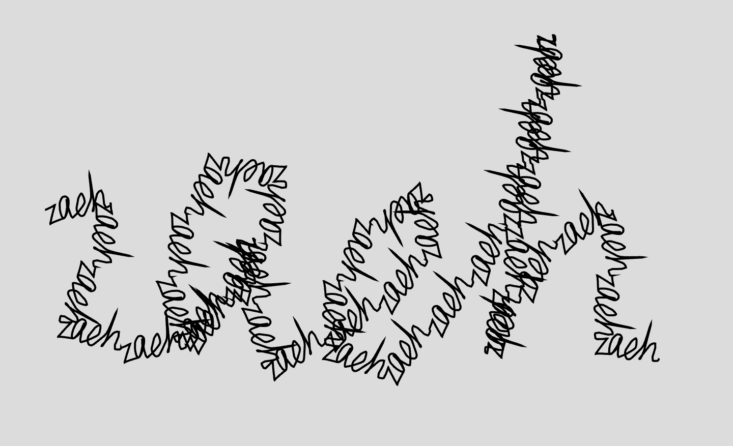
This encoding of line as a binary string allows a direct translation from 1D cellular automaton. As rule 110 of 1bit, 1D cellular automaton is Turing complete, a Turing complete language can also be made out of a single, wiggling line.
The wiggling of this "worm" might seem somewhat random at first, but over time one might discover it to possess some sort of "intelligence", as semi-repeating patterns start to emerge, as if working toward a certain end. This is due to the nature of class 4 cellular automatons, also exhibited in Game of Life and others.
Perhaps the system could be called "Angular Automaton", an alternative visualization of 1D cellular automaton.
Recursion is a powerful concept in programming, though it could be a small challenge for beginners to understand and appreciate. Fractals, though not necessarily recursive, can be seen as a typical and captivating graphical manifestation of recursion. Here we introduce a simple tool to create fractal-like patterns with a single stroke of gesture in real time, without involving code.
The algorithm is quite straightforward. The input polyline is resampled according to certain metric (e.g. equidistant samples). The distance and angle between the first point and the last point are computed. For each two samples, the connecting segment is replaced with a duplicate of the entire polyline, rotated and scaled, such that the endpoints matches these two samples.
The equidistant resampling metric can be replaced with one that produce less samples where the line is smooth, and more where the line has details (polyline simplification, such as Douglas-Peucker). This creates fractals of various different scales, and can be more visually intriguing for certain input patterns.
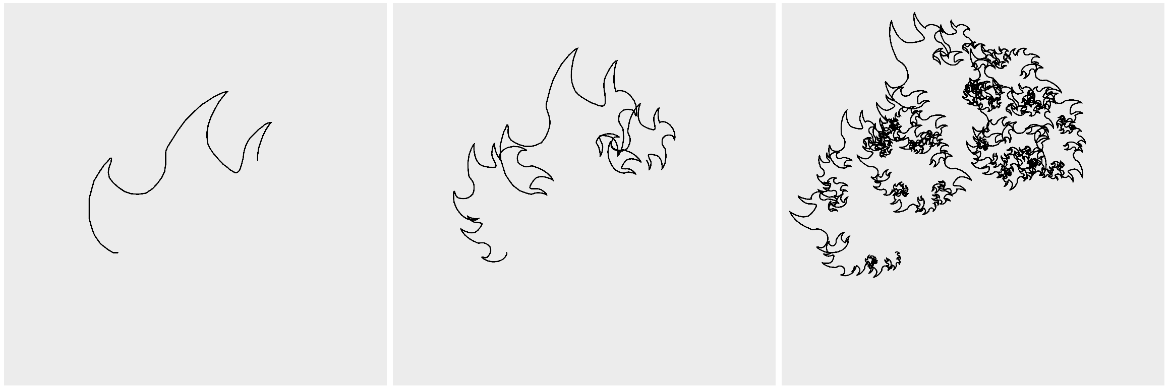
The procedure can be repeated over the output polyline, to create a higher-order fractal, which, can be again used as input, recursively, to create tinier and tinier details. However, optimization would be needed to maintain realtime interactive framerate.
Though the mechanism is simple, it often produces interesting and unexpected visuals.
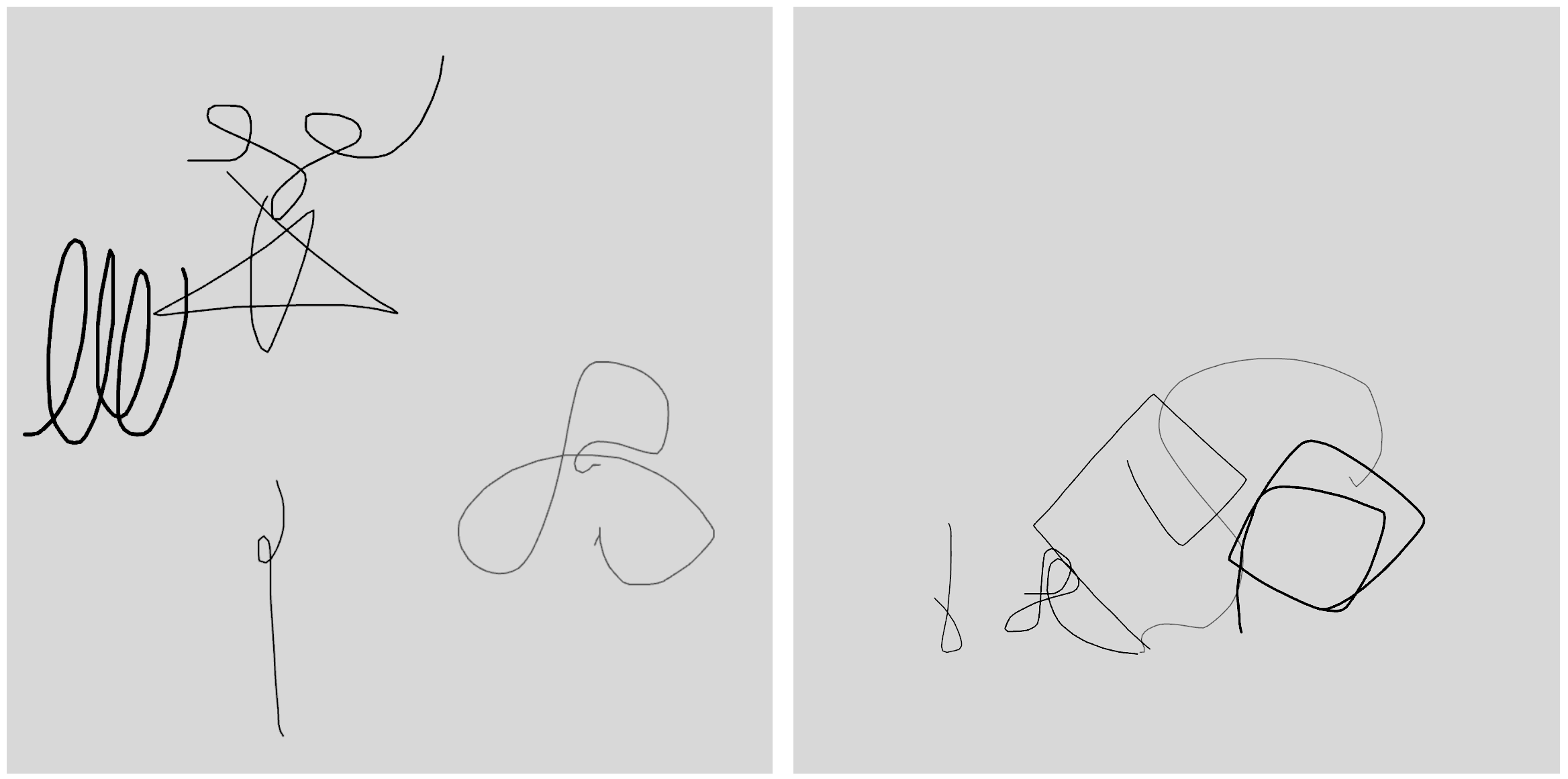
Amongst Prof. Zach Lieberman's pedagogical examples, is a simple yet charming interactive animation: the user draws a single stroke, and the animation "uncurls" the line until it becomes straight, and "curls" it in the other direction; the motion is repeated back and fro.
The animation is the result of encoding the segments of the polyline as a series of offsets and angle changes, in the coordinate system of the sample before each sample, as illustrated in the following pseudo-code:
function deconstruct(Line){
	let Curv = [];
	for (let i = 0; i < Line.length; i++){
		if (!i){
			Curv.push([...Line[i]]);
			continue;
		}
		let dx = Line[i][0]-Line[i-1][0];
		let dy = Line[i][1]-Line[i-1][1];
		Curv.push([atan2(dy,dx),Math.hypot(dy,dx)]);
	}
	return Curv;
}

function reconstruct(Curv, t){
	let Line = [[...Curv[0]]];
	let aa = 0;
	for (let i = 1; i < Curv.length; i++){
		let [a,l] = Curv[i];
		let a0 = 0;
		if (i>1){
			a0 = Curv[i-1][0];
		}
		let ad = a-a0;
		if (ad < -PI) ad += PI*2;
		if (ad >  PI) ad -= PI*2;
		aa += (ad)*cos(t*PI/period);
		let [x0,y0] = Line[i-1];
		Line.push([x0+cos(aa)*l, y0+sin(aa)*l]);
	}
	return Line;
}
This section introduces several possible "extensions" to this example, that explores programming-like potentials of this interaction.
By putting simple physic simulations on the line, such as gravity and friction, we can create a moving "organism" out of the line that crawls along the bottom of the screen using the curling and uncurling motions.
The uncurling motion is given a small, inertia-like variation, such that it is not entirely symmetrical to the curling motion; This is to prevent the latter from completely undoing the former in terms of crawling by "scratching" against the floor in many situations.
It is interesting to observe how differently drawn lines create organisms that move in strange and unexpected ways. It is also possible to turn this into a game, where the players attempt to draw lines that move the fastest. It is a race of lines.
Consider the case where multiple uncurling lines are placed next to each other ― as they swing, they'll intersect with one another; If we plot out the intersections, the trail would also be lines, which can be subject to the uncurling animation again. Thus, uncurling lines can "reproduce" by intersecting with one another, creating a new generation of lines in each iteration.
Below is a simple algorithm for reconstructing the most likely lines from a series of intersecting points. It does not handle degenerate cases (e.g. when two lines almost coincide).
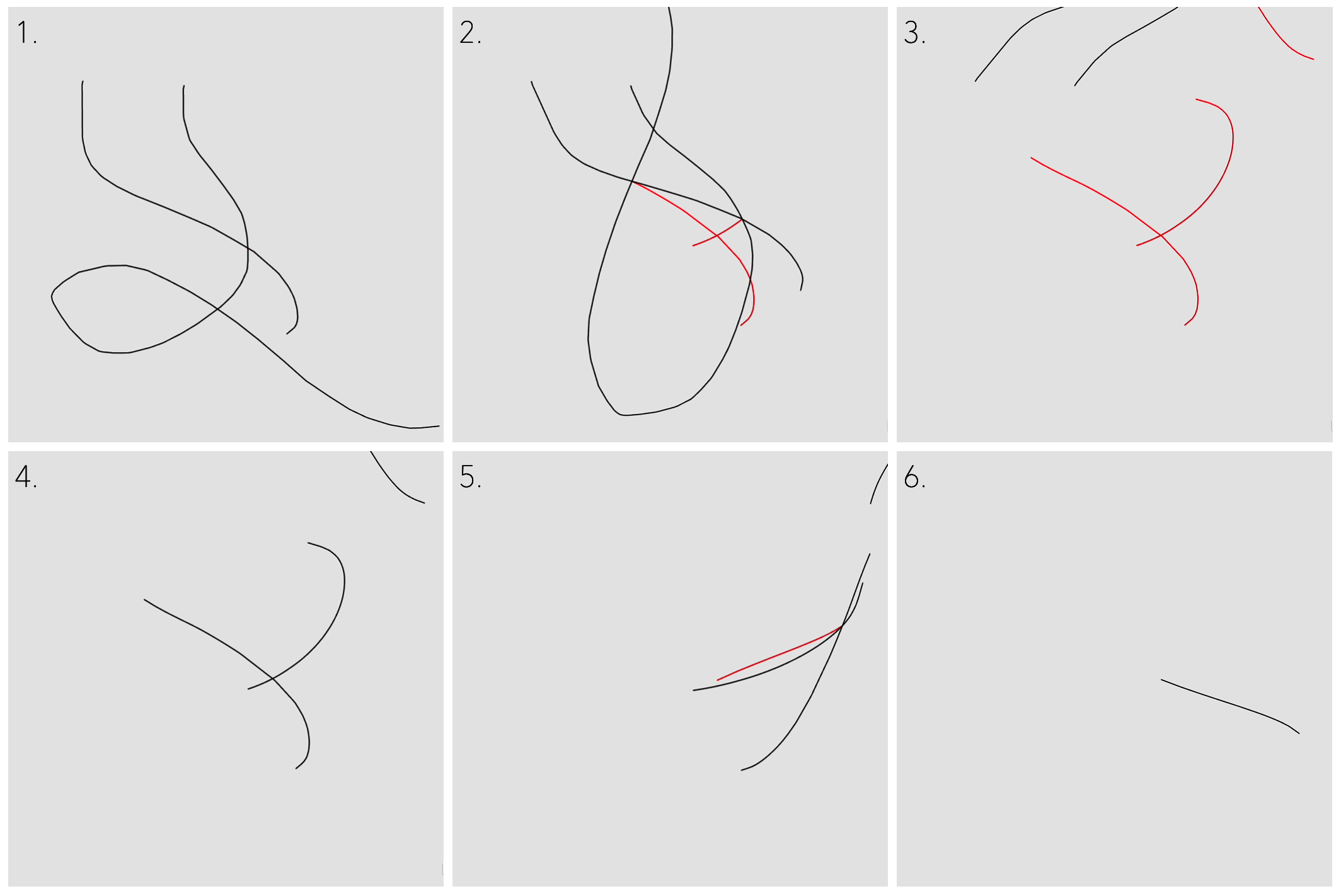
Often times, after a couple generations, there would be either too many lines produced (slowing it to a halt), or there would be not enough lines to produce the next generation ("end of the line", literally). But from time to time carefully crafted inputs can produce long and entertaining animations.
While λ-2D and Nor-wires used the somewhat-beaten "circuit" metaphor, the simple idea of "a dot traveling along a line", being an intuitive and playful concept (compared to static diagrams), nevertheless seems still interesting to explore. This section introduces a few less-circuit-like approaches.
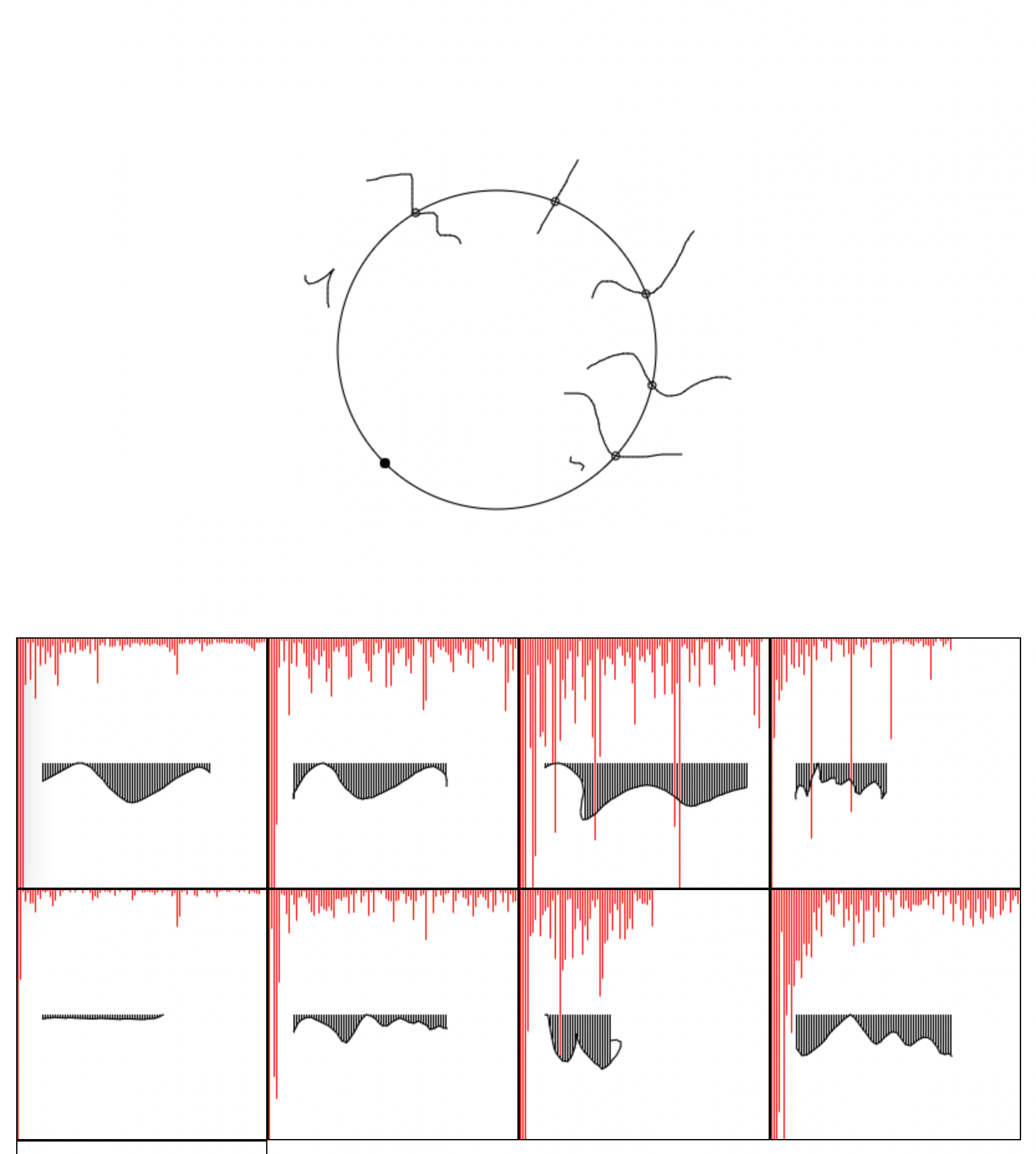
In this experiment, as a dot travels along a line, it can emit a "ray" toward a certain direction. When two of these rays intersect each other, a mark is made at the points of intersection, over time leaving a trail.
For a dot, the color and the direction of its ray can be changed at "nodes". The logic of each node (what it does to incoming dot(s) and input/output directions) is encoded in 24 bits; Therefore each node can be represented by a true color (RGB, 8 bit per channel). Node logic also includes capabilities for generating new dots as well as conditional branching based on the current color of the dot. The color of the dot is encoded as 3 bits (RGB, 1 bit per channel), which can also double as a number from 0-8 and be used for computations. Dots used for this purpose can have their ray-emitting capability turned off.
The simplest usage of the language, is to generate graphics by decomposing 2D motion into two axes, and have motion on each axis be generated by a dot traveling along a crafted path. For example, a 2D circle can be decomposed into two 1D wavy lines on X and Y axes. More complex programs can also be composed, in theory.
In this experiment, a dot travels along a circle, looping indefinitely. With the cursor, the user can draw a squiggly line that crosses the circle. When the dot hits the squiggle, it'll make a noise, and turn back. The squiggle becomes slightly shorter after the impact, until it eventually disappears after many collisions with the dot.
If the user draws a continuous squiggle passing the circle many times, it'll be automatically be split up at maximum turning points.
The frequency and timbre of the sound is determined by the shape of the squiggle. The user literally draws the waveform, which is copied to the sound card. The dot can be trapped between two squiggles, so it bounces back and forth making repeating sounds. Theoretically one can create interesting compositions with this tool.
Instead of rating the languages described in this thesis on a linear scale from "success" to "massive success", each language is given an approximate coordinate in a multidimensional space for their various qualities, strengths and weaknesses. Pairs of qualities that are likely to pose design challenges are plotted against each other (for example, the size of an apartment on X-axis against its rent on Y-axis, falling below a certain line would indicate "a good deal", if other factors such as location are controlled).
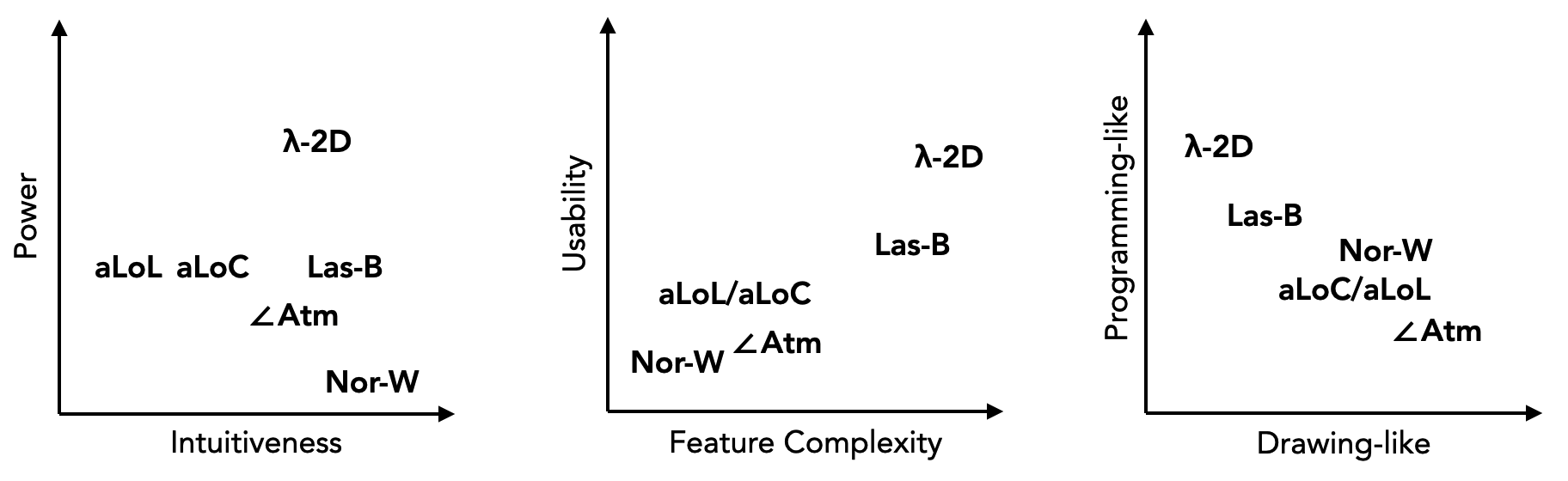
The first plot is intuitiveness v.s. power. Intuitiveness is about how easily a complete beginner can gain a minimal understanding and start experimenting. Power is about how much an experienced user will be able to achieve, what is the maximally complex program that can be written. For example, Microsoft Paint is very intuitive, anyone with a mouse can start doodling in it; GLSL is a lot harder to get started, it takes considerable effort to even get anything to show on screen. However, one would need to be pretty crazy to paint their next masterpiece in MS Paint, whereas an experienced shader programmer can create visually stunning effects and fully leverage the power of the GPU.
The second plot is feature complexity v.s. usability. Feature complexity is about how many features the system has (more does not always mean better). Usability is about how convenient the system is for general purpose programming. Systems with few features yet high usability might be described as "expressive". For example, the C language doesn't have too many features, and is fairly usable. Python and C++ have huge number of extra features, yet usability is only increased moderately in comparison.
The third plot is drawing-like v.s. programming-like. These are about how the experience of using the language feels like. Less programming-like does not necessarily mean more drawing-like. For example, the act of sleeping is neither drawing-like nor programming-like (unless one is dreaming about writing code, of course).
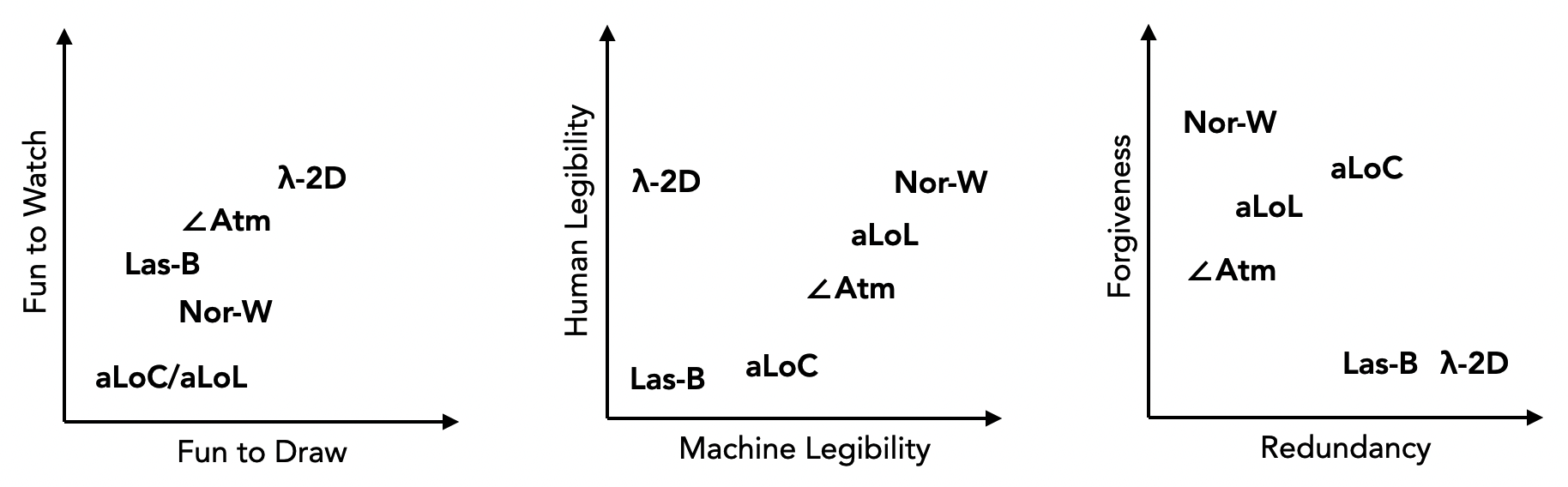
The fourth plot is fun-to-draw v.s. fun-to-watch. These are about how enjoyable it is to create programs in the language, and how enjoyable it is to watch the animation of the program being executed (a feature that exists for most systems described in this document). A wrestling match can be somewhat entertaining to watch, but likely causes some pain for at least one of the contestants.
The fifth plot is machine legibility v.s. human legibility. Machine legibility is about how easy it is for a computer vision algorithm to parse a program; Human legibility is about how easy it is for a human to read and understand the program. For example, QR codes have very high machine legibility, yet are complete mysteries to untrained human eye. Some cursive writing styles have very low legibility for both humans and computers; printed characters are very easy to recognize for humans, while posing a moderate challenge for OCR.
The sixth plot is redundancy v.s. forgiveness. Redundancy is about how verbose the system is, in regard to the information conveyed. Forgiveness is how sloppily the user can use the system, yet still creates valid inputs.
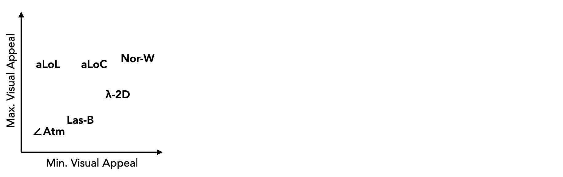
The seventh plot is minimum visual appeal v.s. maximum visual appeal, measuring how interesting the representation of the program itself can look. For example, a stamp's minimum visual appeal approximately equals its maximum visual appeal, as every time it is stamped the imprint looks pretty much the same; In contrast, clay can be shaped to resemble either a nondescript glob, or the finest sculpture.
This thesis describes several drawing-based programming languages, as well as a few programming-like drawing tools. While it is no doubt proved that using drawing as programming language is feasible (and fun), it remains a challenge to design languages that are both simple and intuitive to draw, and powerful enough to create high-level programs conveniently on par with current, text-based languages. It can be argued though, that complexity is inherently complex, and using simple systems to describe complex ones inevitably involves trade-offs. Indeed, each of the systems in this thesis provides some form of trade-off between desirable qualities of "drawing as programming language", whether it is usability, playfulness, or visual appeal.
It can perhaps also be said that, each of the languages, taking distinct visual forms, offers different insights into the structure, patterns and logical flow of programs, which are otherwise difficult to see or visualize for linear, text-based languages. The ability to animate the execution
It is the author's hope that, these experiments as a whole presents a useful collection of novel approaches, and, more importantly, interesting methods of approach to the area of research.
The work is far from done. This thesis is but a peek into the wonderful potentials of drawing as programming language:
Thinking superficially ― how can these drawing-based ideas be integrated into today's programming tools and frameworks, to be of help to the average creative programmer? Such additions would certainly be exciting for areas such as animation and parametric design.
Thinking broadly ― what other new esoteric languages, drawing-based or otherwise, can grow or draw inspiration from these experiments? I envision a world where not only everyone is a programmer (in a broad sense), but also every programmer is a programming language designer (in a broad sense): tried-and-true pre-existing tools are always nice, but it is often the curiosity and the wackiness in experimental tools that drives creativity, which in turn inspires and refines tools of productivity.
Thinking radically ― Lambda calculus, boolean algebra, cellular automaton... they're all existing systems, translated here into a visual and drawing-based form ― Could there be a completely new system, never seen before, specifically ingrained into the nature of drawings? A system that entirely moves away from text, and into the hands and the body, the endless nuances of gestural motions found in drawings? Would this make computing and computational ideas more accessible to everyone? And could there be a program, that can only be so easily and efficiently drawn, but nearly impossible to describe in conventional languages? What would it be like, to forgo all speech and associated intelligence, and start building a programming language from the very beginning? What would they create, if we were to ask the cavemen of Lascaux to design a programming language for us? Would they be able to understand lambda calculus, or what systems would they come up with? What would be the codebase for an operating system look like, as a drawing? Perhaps a great mural on a mile-long wall? How then, could we build such a computer to execute this great mural?